Download
1 / 119
1.2k likes | 1.33k Views
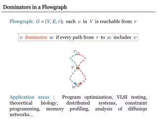
Dominators in a Flowgraph. Flowgraph : G = ( V, E, r ) ; each v in V is reachable from r. v dominates w if every path from r to w includes v.

E N D
Dominators in a Flowgraph Flowgraph: G =(V, E, r); each v in V is reachable from r vdominateswif every path from rtow includes v Application areas : Program optimization, VLSI testing, theoretical biology, distributed systems, constraint programming, memory profiling, analysis of diffusion networks…
Dominators in a Flowgraph Flowgraph: G =(V, E, r); each v in V is reachable from r vdominateswif every path from rtow includes v Set of dominators:Dom(w)={v|v dominates w} Trivial dominators: wr,w,rDom(w) Immediate dominator: idom(w)Dom(w) – w and dominatedby everyv in Dom(w) – w Goal: Find idom(v)for each vinV
Dominators in a Flowgraph Flowgraph: G =(V, E, r); each v in V is reachable from r vdominateswif every path from rtow includes v dominator tree of algorithm: [Lengauer and Tarjan ’79] algorithms: [Alstrup, Harel, Lauridsen, and Thorup ‘97] [Buchsbaum, Kaplan, Rogers, and Westbrook ‘04] [G., and Tarjan ‘04] [Buchsbaumet al. ‘08]
Application: Loop Optimizations Loop optimizations typically make a program much more efficient since a large fraction of the total running time is spent on loops. Dominators can be used to detect loops.
Application: Loop Optimizations Loop L • There is a node h L(loop header), such that • There is a (v,h) for some vL • For any w L-hthere is no (v,w) for vL • h is reachable from every w L • h reaches every w L h a b c d e Thus h dominates all nodes in L. Loop back-edge: (v,h) A and h dominates v.
Application: Identifying Functionally Equivalent Faults x1 Consider a circuit C: Inputs: x1, … , xn Output: f(x1, … ,xn) Suppose there is a fault in wire a.ThenC = Caevaluatesfainstead. Fault a and fault b are functionally equivalent iff fa(x1, … ,xn) = fb(x1, … ,xn) Such pairs of faults are indistinguishable and we want to avoid spending time to distinguish them (since it is impossible). x2 x3 b x4 fb x5
Application: Identifying Functionally Equivalent Faults a x1 Consider a circuit C: Inputs: x1, … , xn Output: f(x1, … ,xn) Suppose there is a fault in wire a.ThenC = Caevaluatesfainstead. Fault a and fault b are functionally equivalent iff fa(x1, … ,xn) = fb(x1, … ,xn) It suffices to evaluate the output of a gate g that dominates a and b. This is can be faster than evaluating f since g may have fewer inputs. g x2 x3 b x4 f x5
Example r Dom(r)={r } Dom(b)={r, b } Dom(c)={r, c } Dom(a)={r, a } Dom(d)={r, d } Dom(e)={r, e } Dom(l)={r, d, l } Dom(h)={r, h } c b g a d e f l j h i k
Example Dom(r)={r } Dom(b)={r, b } Dom(c)={r, c } Dom(a)={r, a } Dom(d)={r, d } Dom(e)={r, e } Dom(l)={r, d, l } Dom(h)={r, h } Dom(k)={r, k } Dom(f)={r, c, f } Dom(g)={r, g } r c b g a d e f l j h i k
Example Dom(b)={r, b } Dom(c)={r, c } Dom(a)={r, a } Dom(d)={r, d } Dom(e)={r, e } Dom(l)={r,d, l } Dom(h)={r, h } Dom(k)={r, k } Dom(f)={r,c, f } Dom(g)={r, g } Dom(j)={r,g, j } Dom(i)={r, i } r c b g a d e f l j h i k
Example idom(b)=r idom(c)=r idom(a)=r idom(d)=r idom(e)=r idom(l)=d idom(h)=r idom(k)=r idom(f)=c idom(g)=r idom(j)=g idom(i)=r r c b g a d e f l j h i k
Example r r g i e a b c d h k c b g a j f l d e f Dominator Tree D D=(V,w r(idom(w),w)) l j h i k
A Straightforward Algorithm Purdom-Moore [1972]: for all vinV– r do remove vfromG R(v) unreachable vertices for alluinR(v) do Dom(u)Dom(u) { v } done done The running time is O(nm).Also very slow in practice.
Iterative Algorithm Dominators can be computed by solving iteratively the set of equations [Allen and Cocke, 1972] Initialization In the intersection we consider only the nonempty Dom(u). Each Dom(v)set can be represented by an n-bit vector. Intersection bit-wise AND. Requires n2space. Very slow in practice (but better than PM).
Iterative Algorithm Dominators can be computed by solving iteratively the set of equations [Allen and Cocke, 1972] Efficient implementation [Cooper, Harvey and Kennedy 2000]: Maintain tree ; process the edges until a fixed-pointis reached. Process : compute nearest common ancestor of and in . If is ancestor of parent of , make new parent of .
Iterative Algorithm Efficient implementation [Cooper, Harvey and Kennedy 2000] dfs(r) T {r} changed true while (changed ) do changed false for all vinV– r in reverse postorderdo x nca(pred(v)) if x parent(v)then parent(v)x changed true end done done
Iterative Algorithm: Example Perform a depth-first search on G postorder numbers r r 13 c 6 b c 12 b g e a g 4 5 8 11 f a d e f 3 7 d 10 j h l j i 9 2 l h i k 1 k
r 13 c 6 b 12 e g 4 5 8 a 11 f 3 7 d 10 j h i 9 2 l k 1 Iterative Algorithm: Example iteration = 1 process 12
r 13 c 6 b 12 e g 4 5 8 a 11 f 3 7 d 10 j h i 9 2 l k 1 Iterative Algorithm: Example iteration = 1 process 11
r 13 c 6 b 12 e g 4 5 8 a 11 f 3 7 d 10 j h i 9 2 l k 1 Iterative Algorithm: Example iteration = 1 process 11
r 13 c 6 b 12 e g 4 5 8 a 11 f 3 7 d 10 j h i 9 2 l k 1 Iterative Algorithm: Example iteration = 1 process 10
r 13 c 6 b 12 e g 4 5 8 a 11 f 3 7 d 10 j h i 9 2 l k 1 Iterative Algorithm: Example iteration = 1 process 7
r 13 c 6 b 12 e g 4 5 8 a 11 f 3 7 d 10 j h i 9 2 l k 1 Iterative Algorithm: Example iteration = 1 process 1
r 13 c 6 b 12 e g 4 5 8 a 11 f 3 7 d 10 j h i 9 2 l k 1 Iterative Algorithm: Example iteration = 2 process 8
r 13 c 6 b 12 e g 4 5 8 a 11 f 3 7 d 10 j h i 9 2 l k 1 Iterative Algorithm: Example iteration = 2 process 8
r 13 c 6 b 12 e g 4 5 8 a 11 f 3 7 d 10 j h i 9 2 l k 1 Iterative Algorithm: Example iteration = 2 process 2
r 13 c 6 b 12 e g 4 5 8 a 11 f 3 7 d 10 j h i 9 2 l k 1 Iterative Algorithm: Example iteration = 2 process 2
r 13 c 6 b 12 e g 4 5 8 a 11 f 3 7 d 10 j h i 9 2 l k 1 Iterative Algorithm: Example iteration = 3 process 4
r 13 c 6 b 12 e g 4 5 8 a 11 f l 9 3 7 d 10 j h i 2 k 1 Iterative Algorithm: Example iteration = 3 process 4 DONE! But we need one more iteration to verify that nothing changes
r 13 6 c b 12 e g 5 8 4 a 11 f 3 7 d 10 j h i 9 2 l k 1 Iterative Algorithm Running Time Each pairwise intersection takes O(n) time. #iterations d + 3. [Kam and Ullman 1976] d =max#back-edges in any cycle-free path of G d = 2
Iterative Algorithm Running Time Each pairwise intersection takes O(n) time. The number of iterations is d + 3. d =max#back-edges in any cycle-free path of G = O(n) Running time = O(mn2) This bound is tight, but very pessimistic in practice.
A Fast Dominator Algorithm Lengauer-Tarjan [1979]:O(m(m,n))time A simpler version runs inO(m log 2+ m/n n)time
The Lengauer-Tarjan Algorithm: Depth-First Search Perform a depth-first search on G DFS-tree T r r 1 c 2 b c 8 b g e a g 3 7 9 11 f a d e f 4 10 d 12 j h l j i 13 5 l h i k 6 k
The Lengauer-Tarjan Algorithm: Depth-First Search Depth-First Search Tree T: We refer to the vertices by their DFS numbers: v<w :v was visited by DFS before w Notation v*w:vis an ancestor of winT v+w:vis a proper ancestor of winT parent(v) : parent of vinT Property 1 v,wsuch that vw,(v,w)Ev*w
The Lengauer-Tarjan Algorithm: Semidominators Semidominator path (SDOM-path): P= (v0=v,v1,v2, …,vk=w)such that vi>w, for 1 ik-1 (r, a,d, l ,h, e) is an SDOM-path for e r 1 c 2 b 8 e g 3 7 9 11 f a 4 10 d 12 j h i 13 5 l k 6
The Lengauer-Tarjan Algorithm: Semidominators Semidominator path (SDOM-path): P= (v0=v,v1,v2, …,vk=w)such that vi>w, for 1 ik-1 Semidominator: sdom(w)= min {v|SDOM-pathfromvtow} r 1 c 2 b 8 e g 3 7 9 11 f a 4 10 d 12 j h i 13 5 l k 6
The Lengauer-Tarjan Algorithm: Semidominators Semidominator path (SDOM-path): P= (v0=v,v1,v2, …,vk=w)such that vi>w, for 1 ik-1 Semidominator: sdom(w)= min {v|SDOM-pathfromvtow} r 1 c 2 b 8 sdom(e)=r e g 3 7 9 11 f a 4 10 d 12 j h i 13 5 l k 6
The Lengauer-Tarjan Algorithm: Semidominators • For any w r,idom(w) * sdom(w)+ w. idom(w) sdom(w) w
The Lengauer-Tarjan Algorithm: Semidominators • For any w r,idom(w) * sdom(w)+ w. • sdom(w) = min ( { v | (v, w) E and v<w } • {sdom(u)|u>wand(v, w)Esuch thatu *v}). sdom(u) sdom(u) nca(w,v) = v nca(w,v) = w nca(w,v) w u w u v v
The Lengauer-Tarjan Algorithm: Semidominators • For any w r,idom(w) * sdom(w)+ w. • sdom(w) = min ( { v | (v, w) E and v<w } • {sdom(u)|u>wand(v, w)Esuch thatu *v}). • Letwr and let ube any vertex with minsdom(u) that • satisfies sdom(w)+u*w. Then idom(w)=idom(u). sdom(u) sdom(w) idom(w) = idom(u) u w
The Lengauer-Tarjan Algorithm: Semidominators • For any w r,idom(w) * sdom(w)+ w. • sdom(w) = min ( { v | (v, w) E and v<w } • {sdom(u)|u>wand(v, w)Esuch thatu *v}). • Letwr and let ube any vertex with minsdom(u) that • satisfies sdom(w)+u*w. Then idom(w)=idom(u). • Moreover, if sdom(u)=sdom(w)thenidom(w)=sdom(w). sdom(u) = sdom(w) idom(w) = sdom(w) u w
The Lengauer-Tarjan Algorithm • Overview of the Algorithm • Carry out a DFS. • Process the vertices in reverse preorder. For vertex • w, compute sdom(w). • Implicitly define idom(w). • Explicitly define idom(w)by a preorder pass.
Evaluating minima on tree paths If we process vertices in reverse preorderthen the sdom values we need are known.
Evaluating minima on tree paths Data Structure: Maintain forest F and supports the operations: link(v,w): Add the edge (v,w)to F. eval(v): Let r be the root of the tree that contains v in F. If v= r then return v. Otherwise return any vertex with minimum sdom among the vertices uthat satisfy r+u*v. Initially every vertex in V is a root in F.
The Lengauer-Tarjan Algorithm dfs(r) for allwVin reverse preorder do for allvpred(w)do ueval(v) ifsemi(u)<semi(w)thensemi(w)semi(u) done add w to the bucket of semi(w) link(parent(w),w) for allvin the bucket of parent(w)do delete vfrom the bucket of parent(w) ueval(v) ifsemi(u)<semi(v)thendom(v)u elsedom(v)parent(w) done done for allwVin reverse preorder do ifdom(w)semi(w)thendom(w)dom(dom(w)) done
r 1 c 2 b 8 e g 3 7 9 a 11 f 4 10 d 12 j h i 13 5 l k 6 The Lengauer-Tarjan Algorithm: Example
r 1 c 2 b 8 e g 3 7 9 a 11 f 4 10 d 12 j h i 13 5 l k 6 The Lengauer-Tarjan Algorithm: Example eval(12) = 12 [12]
r 1 c 2 b 8 e g 3 7 9 a 11 f 4 10 d 12 j h i 13 5 l k 6 The Lengauer-Tarjan Algorithm: Example add 13 to bucket(12) link(13) 13 [12]
r 1 c 2 b 8 e g 3 7 9 a 11 f 4 10 d 12 j h i 13 5 l k 6 The Lengauer-Tarjan Algorithm: Example delete 13 from bucket(12) eval(13) = 13 dom(13)=12 [12]
r 1 c 2 b 8 e g 3 7 9 a 11 f 4 10 d 12 j h i 13 5 l k 6 The Lengauer-Tarjan Algorithm: Example eval(11) = 11 [11] dom(13)=12 [12]