Download
1 / 74
2.38k likes | 4.32k Views
Chapter 3: Image Enhancement in the Spatial Domain. 3.1 Background 3.2 Some basic intensity transformation functions 3.3 Histogram processing 3.4 Fundamentals of spatial filtering 3.5 Smoothing spatial filters 3.6 Sharpening spatial filters. Preview.

E N D
Chapter 3: Image Enhancement in the Spatial Domain 3.1 Background 3.2 Some basic intensity transformation functions 3.3 Histogram processing 3.4 Fundamentals of spatial filtering 3.5 Smoothing spatial filters 3.6 Sharpening spatial filters
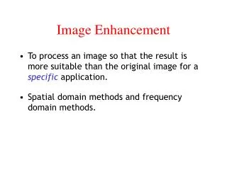
Preview • Spatial domain processing: direct manipulation of pixels in an image • Two categories of spatial (domain) processing • Intensity transformation: • Operate on single pixels • Contrast manipulation, image thresholding • Spatial filtering • Work in a neighborhood of every pixel in an image • Image smoothing, image sharpening
3.1 Background • Spatial domain methods: operate directly on pixels • Spatial domain processing • g(x,y) = T[f(x, y)] • f(x, y): input image • g(x, y): output (processed) image • T: operator • Operator T is defined over a neighborhood of point (x, y)
3.1 Background Spatial filtering • For any location (x,y), output image g(x,y) is equal to the result of applying T to the neighborhood of (x,y) in f • Filter: mask, kernel, template, window
3.1 Background • The simplest form of T: g depends only on the value of f at (x, y) • T becomes intensity (gray-level) transformation function • s = T(r) • r: intensity of f(x,y) • s: intensity of g(x,y) • Point processing: enhancement at any point depends only on the gray level at that point
3.1 Background Point processing • (a) Contrast stretching • Values of r below k are compressed into a narrow range of s • (b) Thresholding
3.2 Some Basic Intensity Transformation Functions • r: pixel value before processing • s: pixel value after processing • T: transformation • s = T(r) • 3 types • Linear (identity and negative transformations) • Logarithmic (log and inverse-log transformations) • Power-law (nth power and nth root transformations)
3.2.1 Image Negatives • Negative of an image with gray level [0, L-1] • s = L – 1 – r • Enhancing white or gray detail embedded in dark regions of an image
3.2.2 Log Transformations • General form of log transformation • s = c log(1+r) • c: constant, r ≥ 0 • This transformation maps a narrow range of low gray-level values in the input image into a wider range of output levels • Classical application of log transformation: • Display of Fourier spectrum
3.2.2 Log Transformations • (a) Original Fourier spectrum: 0 ~ 1,500,000 range • scaled to 0 ~ 255 • (b) Result of log transformation: 0 ~ 6.2 range • scaled to 0 ~ 255
3.2.3 Power-Law Transformations • Basic form of power-law transformations • s = c r γ • c, γ: positive constants • Gamma correction: • process of correcting this power-law response • Example: cathode ray tube (CRT) • Intensity to voltage response is power function with exponent (γ) 1.8 to 2.5 • Solution: preprocess the input image by performing transformation • s = r1/2.5 = r0.4
3.2.3 Power-Law Transformations CRT monitor gamma correction example
3.2.3 Power-Law Transformations MRI gamma correction example γ = 0.6 original γ= 0.4 γ= 0.3
3.2.3 Power-Law Transformations Arial image gamma correction example original γ = 3.0 γ = 5.0 γ = 4.0
3.2.4 Piecewise-Linear Transformation Functions Contrast stretching Low contrast image Piecewise linear function Result of contrast stretching Result of thresholding
3.2.4 Piecewise-Linear Transformation Functions Contrast stretching (c) Contrast stretching (r1, s1) = (rmin, 0), (r2, s2) = (rmax, L-1) rmin, rmax: minimum, maxmum level of image (d)Thresholding: r1 = r2 = m, s1 = 0, s2 = L-1 m: mean gray level
3.2.4 Piecewise-Linear Transformation Functions Intensity-level slicing
3.2.4 Piecewise-Linear Transformation Functions Intensity-level slicing • Display a high value for all gray levels in the range of interest, and a low value for all other images • - produces binary image • (b)Brightens the desired range of gray levels • but preserves the background and other parts
3.2.4 Piecewise-Linear Transformation Functions Intensity-level slicing
3.2.4 Piecewise-Linear Transformation Functions Bit-plane slicing
3.2.4 Piecewise-Linear Transformation Functions Bit-plane slicing
3.2.4 Piecewise-Linear Transformation Functions Bit-plane slicing • Multiply bit plane 8 by 128 • Multiply bit plane 7 by 64 • Add the results of two planes
3.3 Histogram Processing • The histogram of digital image with gray levels in the range [0, L-1] is a discrete function • h(rk) = nk • rk: kth gray level • nk: number of pixels in image having gray levels rk • Normalized histogram • p(rk) = nk/n • n: total number of pixels in image • n = MN (M: row dimension, N: column dimension)
3.3 Histogram Processing • Histogram • horizonal axis: • rk(kthintensity value) • vertical axis: • nk: number of pixels, or • nk/n: normalized number
3.3.1 Histogram Equalization • r: intensities of the image to be enhanced • r is in the range [0, L-1] • r = 0: black, r = L-1: white • s: processed gray levels for every pixel value r • s = T(r), 0 ≤ r ≤ L-1 • Requirements of transformation function T • T(r) is a (strictly) monotonically increasing in the interval 0 ≤ r ≤ L-1 • 0 ≤ T(r) ≤ L-1for 0 ≤ r ≤ L-1 • Inverse transformation • r = T-1(s), 0 ≤s ≤L-1
3.3.1 Histogram Equalization Intensity transformation function
3.3.1 Histogram Equalization Intensity levels: random variable in interval [0, L-1] probability density function (PDF) cumulative distribution function (CDF) Uniform probability density function
3.3.1 Histogram Equalization MN: total number of pixels in image nk: number of pixels having gray level rk L: total number of possible gray levels • histogram equalization (histogram linearization): • Processed image is obtained by mapping each pixel rk(input image) • into corresponding level sk (output image)
3.3.1 Histogram Equalization Histogram equalization from dark image (1) Histogram equalization from light image (2) Histogram equalization from low contrast image (3) Histogram equalization from high contrast image (4)
3.3.1 Histogram Equalization Transformation functions
3.3.3 Local Histogram Processing • Histogram processing methods in previous section are global • Global methods are suitable for overall enhancement • Histogram processing techniques are easily adapted to local enhancement • Example • (b) Global histogram equalization Considerable enhancement of noise • (c) Local histogram equalization using 7x7 neighborhood • Reveals (enhances) the small squares inside the dark squares • Contains finer noise texture
3.3.3 Local Histogram Processing Local histogram equalized image Global histogram equalized image Original image
3.3.4 Use of Histogram Statistics for Image Enhancement r: discrete random variable representing intensity values in the range [0, L-1] p(ri): normalized histogram component corresponding to valueri nth moment of r mean (average) value of r variance of r, б2(r) sample mean sample variance
3.3.4 Use of Histogram Statistics for Image Enhancement • Global mean and variance are measured over entire image • Used for gross adjustment of overall intensity and contrast • Local mean and variance are measured locally • Used for local adjustment of local intensity and contrast (x,y): coordinate of a pixel Sxy: neighborhood (subimage), centered on (x,y) r0, …, rL-1: L possible intensity values pSxy: histogram of pixels in region Sxy local mean local variance
3.3.4 Use of Histogram Statistics for Image Enhancement • A measure whether an area is relatively light or dark at (x,y) • Compare the local average gray level mSxy to the global mean mG • (x,y) is a candidate for enhancement if mSxy ≤ k0mG • Enhance areas that have low contrast • Compare the local standard deviation бSxyto the global standard • deviation бG • (x,y) is a candidate for enhancement if бSxy ≤ k2 бG • Restrict lowest values of contrast • (x,y) is a candidate for enhancement if k1 бG≤ бSxy • Enhancement is processed simply multiplying the gray level • by a constant E
3.3.4 Use of Histogram Statistics for Image Enhancement Problem: enhance dark areas while leaving the light area as unchanged as possible E = 4.0, k0 = 0.4, k1 = 0.02, k2 = 0.4, Local region (neighborhood) size: 3x3
3.4 Fundamentals of Spatial Filtering • Operations with the values of the image pixels in the neighborhood • and the corresponding values of subimage • Subimage: filter, mask, kernel, template, window • Values in the filter subimage: coefficient • Spatial filtering operations are performed directly on the pixels • of an image • One-to-one correspondence between • linear spatial filters and filters in the frequency domain
3.4.1 Mechanics of Spatial Filtering • A spatial filter consists of • (1) a neighborhood (typically a small rectangle) • (2) a predefined operation • A processed (filtered) image is generated as the center of • the filter visits each pixel in the input image • Linear spatial filtering using 3x3 neighborhood • At any point (x,y), the response, g(x,y), of the filter • g(x,y) = w(-1,-1)f(x-1,y-1) + w(-1,0)f(x-1,y) + … • + w(0,0)f(x,y) + …+ w(1,0)f(x+1,y) + w(1,1)f(x+1,y+1)
3.4.1 Mechanics of Spatial Filtering • Filtering of an image f with a filter w of size m x n • a = (m-1) / 2, b = (n-1) / 2 or m = 2a+1, n = 2b+1 • (a, b: positive integer)
3.4.2 Spatial Correlation and Convolution • Correlation of a filter w(x,y) of size m x n with an image f(x,y) • Convolution of w(x,y) and f(x,y)
3.4.3 Vector Representation of Linear Filtering • Linear spatial filtering by m x n filter • Linear spatial filtering by 3 x 3 filter
3.4.3 Vector Representation of Linear Filtering • Spatial filtering at the border of an image • Limit the center of the mask no less than (n-1)/2 pixels • from the border -> Smaller filtered image • Padding -> Effect near the border • Adding rows and columns of 0’s • Replicating rows and columns
3.4.4 Generating Spatial Filter Masks • Linear spatial filtering by 3 x 3 filter • Average value in 3 x 3 neighborhood • Gaussian function