Introduction to Natural Language Processing (NLP)

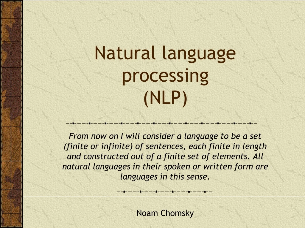
1. Natural language processing(NLP) From now on I will consider a language to be a set (finite or infinite) of sentences, each finite in length and constructed out of a finite set of elements. All natural languages in their spoken or written form are languages in this sense. Noam Chomsky

2. Levels of processing • Semantics • Focuses on the study of the meaning of words and the interactions between words to form larger units of meaning (such as sentences) • Discourse • Building on the semantic level, discourse analysis aims to determine the relationships between sentences • Pragmatics • Studies how context, world knowledge, language conventions and other abstract properties contribute to the meaning of text

3. Evolution of translation

4. NLP • Text is more difficult to process than numbers • A word can have multiple senses and meaning • Set is a verb, noun, and adjective • Language has many irregularities • Typical speech and written text are not perfect • Don’t expect perfection from text analysis

5. Shortcomings • Irony • The name of Britain’s biggest dog (until it died) was Tiny • Sarcasm • I started out with nothing and still have most of it left • Word analysis • “Not happy” scores +1

6. Tokenization • Breaking a document into chunks • Tokens • Typically words • Break at whitespace • Create a “bag of words” • Many operations are at the word level

7. Terminology • N • Corpus size • Number of tokens • V • Vocabulary • Number of distinct tokens in the corpus

8. Count the number of words library(stringr) str_count("The dead batteries were given out free of charge", "[[:space:]]+") + 1

9. Sentiment analysis with R • sentimentr package • Uses a polarity table of words and their weights (e.g., positive words +1, and negative words -1) • Default polarity table is based on Jockers (2017) in syuzhet package. • You can create your own polarity table • Not restricted to -1 and +1

10. Polarity table > library(sentimentr) > library(syuzhet) > head(get_sentiment_dictionary()) word value 1 abandon -0.75 2 abandoned -0.50 3 abandoner -0.25 4 abandonment -0.25 5 abandons -1.00 6 abducted -1.00

11. Valence shifters • Valence shifters alter or intensify the meaning of polarizing words • Negators • Negate a sentence's meaning • "I do not like pie" • Amplifiers • Intensify a sentence's meaning • "I seriously do not like pie" • "I barely like pie"

12. Sentiment analysis library(sentimentr) sample = c("You're awesome and I love you", "I hate and hate and hate. So angry. Die!", "Impressed and amazed: you are peerless in your achievement of unparalleledmediocrity.") sentiment(sample, n.before=0, n.after=0, amplifier.weight=0) element_idsentence_idword_count sentiment 1: 1 1 6 0.5511352 2: 2 1 6 -0.9185587 3: 2 2 2 -0.5303301 4: 2 3 1 -0.7500000 5: 3 1 12 0.6495191 • Each paragraph is broken into sentences, and each sentence is broken into an ordered bag of words • Sentiment score • Sum of word scores/sqrt(word count)

13. Sentiment analysis library(sentimentr) sample = c("You're awesome and I love you", "I hate and hate and hate. So angry. Die!", "Impressed and amazed: you are peerless in your achievement of unparalleledmediocrity.") y <- sentiment(sample, n.before=0, n.after=0, amplifier.weight=0) mean(y$sentiment) [1] -0.1996469 • Overall score

14. Valence shifting sentiment(text, n.before=2, n.after=2, amplifier.weight=.8, but.weight = .9)

15. Exercise sample = c("You're not crazyand I love you very much.") sentiment(sample, n.before = 4, n.after=2, amplifier.weight=1) sentiment(sample, n.before = Inf, n.after=Inf, amplifier.weight=1) Run the following code and comment on how sensitive sentiment analysis is to the n.before and n.after parameters

16. Text mining with tm

17. Creating a corpus while (i < 2013) { y <- as.character(i) # create the file name url <- str_c('http://www.richardtwatson.com/data/BuffettLetters/', y, 'ltr.txt',sep='') # read the letter as on large string d <- read_file(url) # d <- readChar(f,nchars=1e6) d <- gsub("[^[:alnum:]///' ]", " ", d) # get rid of odd characters # add letter to the data frame df[i-begin+1,1] <- y # the letter id df[i-begin+1,2] <- d # the letter i <- i + 1 } colnames(df) <- c('doc_id', 'text') # create the corpus letters <- Corpus(DataframeSource(as.data.frame(df))) A corpus is a collection of written texts Load Warren Buffet’s letters

18. Exercise Create a corpus of Warren Buffet’s letters for 2008-2012

19. Readability • Flesch-Kincaid • An estimate of the grade-level or years of education required of the reader • 13-16 Undergrad • 16-18 Masters • 19 - PhD • (11.8 * syllables_per_word) + (0.39 * words_per_sentence) - 15.59

20. koRpus library(koRpus) library(koRpus.lang.en) #tokenize the first letter in the corpus after converting to character vector txt <- letters[[1]][1] # first element in the list tagged.text <- koRpus::tokenize(as.character(txt),format='obj',lang='en') # score readability(tagged.text, hyphen=NULL,index="FORCAST")

21. Exercise What is the Flesch-Kincaid score for the 2010 letter?

22. Preprocessing • Case conversion • Typically to all lower case • clean.letters <- tm_map(letters, content_transformer(tolower)) • Punctuation removal • Remove all punctuation • clean.letters <- tm_map(clean.letters, content_transformer(removePunctuation)) • Number filter • Remove all numbers • clean.letters <- tm_map(clean.letters, content_transformer(removeNumbers))

23. Convert to lowercase before removing stop words Preprocessing • Strip extra white space • clean.letters <- tm_map(clean.letters, content_transformer(stripWhitespace)) • Stop word filter • clean.letters <- tm_map(clean.letters,removeWords,stopwords('SMART') • Specific word removal • dictionary <- c("berkshire","hathaway", "charlie", "million", "billion", "dollar") • clean.letters <- tm_map(clean.letters,removeWords,dictionary)

24. Preprocessing • Word filter • Remove all words less than or greater than specified lengths • POS (parts of speech) filter • Regex filter • Replacer • Pattern replacer

25. Preprocessing # Sys.setenv(NOAWT = TRUE) # for Mac OS X library(tm) # convert to lower clean.letters <- tm_map(letters, content_transformer(tolower)) # remove punctuation clean.letters <- tm_map(clean.letters,content_transformer(removePunctuation)) # remove numbers clean.letters <- tm_map(clean.letters,content_transformer(removeNumbers)) # strip extra white space clean.letters <- tm_map(clean.letters,content_transformer(stripWhitespace)) # remove stop words clean.letters <- tm_map(clean.letters,removeWords,stopwords('SMART'))

26. Can take a while to run Stemming stem.letters <- tm_map(clean.letters,stemDocument, language = "english") • Reducing inflected (or sometimes derived) words to their stem, base, or root form • Banking to bank • Banks to bank

27. Frequency of words tdm <- TermDocumentMatrix(stem.letters,control = list(minWordLength=3)) dim(tdm) • A simple analysis is to count the number of terms • Extract all the terms and place into a term-document matrix • One row for each term and one column for each document

28. Will take minutes to run Stem completion tdm.stem <- stemCompletion(rownames(tdm), dictionary=clean.letters, type=c("prevalent")) # change to stem completed row names rownames(tdm) <- as.vector(tdm.stem) rownames(tdm)[1:20] • Returns stems to an original form to make text more readable • Uses original document as the dictionary • Several options for selecting the matching word • prevalent, first, longest, shortest • Time consuming so don't apply to the corpus but the term-document matrix

29. Frequency of words • Report the frequency • findFreqTerms(tdm, lowfreq = 100, highfreq = Inf)

30. Exercise • Create a term-document matrix and find the words occurring more than 100 times in the letters for 2008-2102 • Do appropriate preprocessing

31. Frequency • Term frequency (tf) • Words that occur frequently in a document represent its meaning well • Inverse document frequency (idf) • Words that occur frequently in many documents aren’t good at discriminating among documents

32. Frequency of words # convert term document matrix to a regular matrix to get frequencies of words m <- as.matrix(tdm) # sort on frequency of terms to get frequencies of words v <- sort(rowSums(m), decreasing=TRUE) # display the ten most frequent words v[1:10]

33. Exercise • Report the frequency of the 20 most frequent words • Do several runs to identify words that should be removed from the top 20 and remove them

34. Probability density library(ggvis) # get the names corresponding to the words names <- names(v) # create a data frame for plotting d <- data.frame(word=names, freq=v) ggplot(d,aes(freq)) + geom_density(fill="salmon") +xlab("Frequency")

35. Word cloud library(wordcloud) # get the names corresponding to the words names <- names(v) # create a data frame for plotting d <- data.frame(word=names, freq=v) # select the color palette pal = brewer.pal(5,"Accent") # generate the cloud based on the 30 most frequent words wordcloud(d$word, d$freq, min.freq=d$freq[30],colors=pal)

36. Exercise Produce a word cloud for the words identified in the prior exercise

37. Co-occurrence • Co-occurrence measures the frequency with which two words appear together • If two words both appear or neither appears in same document • Correlation = 1 • If two words never appear together in the same document • Correlation = -1

38. Co-occurrence data <- c("word1", "word1 word2","word1 word2 word3","word1 word2 word3 word4","word1 word2 word3 word4 word5") frame <- data.frame(data) frame test <- Corpus(DataframeSource(frame)) tdmTest <- TermDocumentMatrix(test) findFreqTerms(tdmTest)

39. Note that co-occurrence is at the document level Co-occurrence matrix Document > # Correlation between word2 and word3, word4, and word5 > cor(c(0,1,1,1,1),c(0,0,1,1,1)) [1] 0.6123724 > cor(c(0,1,1,1,1),c(0,0,0,1,1)) [1] 0.4082483 > cor(c(0,1,1,1,1),c(0,0,0,0,1)) [1] 0.25

40. Association Measuring the association between a corpus and a given term Compute all correlations between the given term and all terms in the term-document matrix and report those higher than the correlation threshold

41. Find Association Computes correlation of columns to get association # find associations greater than 0.1 findAssocs(tdmTest,"word2",0.1)

42. Find Association shoot cigarettes eyesight pinpoint ringmaster suffice tunnels unnoted 0.83 0.81 0.81 0.81 0.81 0.81 0.81 0.81 # compute the associations findAssocs(tdm, "invest",0.80)

43. Exercise • Select a word and compute its association with other words in the Buffett letters corpus • Adjust the correlation coefficient to get about 10 words

44. Cluster analysis • Assigning documents to groups based on their similarity • Google uses clustering for its news site • Map frequent words into a multi-dimensional space • Multiple methods of clustering • How many clusters?

45. Clustering • The terms in a document are mapped into n-dimensional space • Frequency is used as a weight • Similar documents are close together • Several methods of measuring distance

46. Cluster analysis # Cluster analysis # name the columns for the letter's year colnames(tdm) <- 1998:2012 # Remove sparse terms tdm1 <- removeSparseTerms(tdm, 0.5) # transpose the matrix tdmtranspose <- t(tdm1) cluster = hclust(dist(tdmtranspose)) # plot the tree plot(cluster)

47. Cluster analysis

48. Exercise Review the documentation of the hclust function in the stats package and try one or two other clustering techniques

49. Topic modeling Goes beyond the independent bag-of-words approach to consider the order of words Topics are latent (hidden) The number of topics is fixed in advance Input is a document term matrix

50. Topic modeling • Some methods • Latent Dirichlet allocation (LDA) • Correlated topics model (CTM)