Sampling Design, Spatial Allocation, and Proposed Analyses
260 likes | 287 Views
Sampling Design, Spatial Allocation, and Proposed Analyses. Don Stevens Department of Statistics Oregon State University. Sampling Environmental Populations. Environmental populations exist in a spatial matrix

Sampling Design, Spatial Allocation, and Proposed Analyses
E N D
Presentation Transcript
Sampling Design, Spatial Allocation, and Proposed Analyses Don Stevens Department of Statistics Oregon State University
Sampling Environmental Populations • Environmental populations exist in a spatial matrix • Population elements close to one another tend to be more similar than widely separated elements • Good sampling designs tend to spread out the sample points more or less regularly • Simple random sampling (SRS) tends to result in point patterns with voids and clusters of points
Sampling Environmental Populations • Systematic sample has substantial disadvantages • Well known problems with periodic response • Less well recognized problem: patch-like response • Inflexible point density doesn’t accommodate • Adjustment for frame errors • Sampling through time
Random-tessellation Stratified (RTS) Design • Compromise between systematic & SRS that resolves periodic/patchy response • Cover the population domain with a randomly placed grid • Select one sample point at random from each grid cell
RTS Design • Does not resolve systematic sample difficulties with • variable probability (point density) • unreliable frame material • Sampling through time
Generalized Random-tessellation Stratified (GRTS) Design • Design is based on a random function that maps the unit square into the unit interval. • The random function is constructed so that it is 1-1 and preserves some 2-dimensional proximity relationships in the 1-dimensional image. • Accommodates variable sample point density, sample augmentation, and spatially-structured temporal samples.
Spatial Properties Of Reverse Hierarchical Ordered GRTS Sample • The complete sample is nearly regular, capturing much of the potential efficiency of a systematic sample without the potential flaws. • Any subsample consisting of a consecutive subsequence is almost as regular as the full sample; in particular, the subsequence. , is a spatially well-balanced sample. • Any consecutive sequence subsample, restricted to the accessible domain, is a spatially well-balanced sample of the accessible domain (critical for sediment sample).
Spatially Balanced Sample • Assess spatial balance by variance of size of Voronoi polygons, compared to SRS sample of the same size. • Voronoi polygons for a set of points: The ith polygon is the collection of points in the domain that are closer to si than to any other sj in the set.
Sampling Through Time • Detection of a signal that is small relative to noise magnitude requires replication • Spatial replication (more samples per year) addresses spatial variation • Need temporal replication (more years) to address temporal variation • Detection of trend in slowly changing status requires many years
Sampling Through Time • Repeat sampling of same site eliminates a variance component if the site retains its identity through time. • Design based on assumption that sediment does retain identity, but water does not. • Both water and sediment samples have spatial balance through time, but sediment sample includes revisits at 1, 5, and 10 year intervals.
Proposed Analyses • Annual descriptive summaries • Mean values, proportions, distributions, precision estimates based on annual data • Mean concentration confidence limits • Percent area in non-compliance confidence limits • Histograms • Distribution function plots confidence limits • Subpopulation comparisons
Proposed Analyses • Composite estimation: Annual status estimates that incorporate prior data • Model that predicts current value at site s based on prior observation: • Composite estimator is weighted combination of mean of current observation and mean of predicted values based on prior observations • Results in increased precision for annual estimates • Can also be used to “borrow strength” from spatially proximate data
Proposed Analyses • Trend Analyses. • Need to describe trend at the segment or Bay level. • Usual approach: trend in mean value. • Also consider: trend in spatial pattern, trend in population distribution, distribution of trend, and mean value of trend. • Trend analyses will exploit repeat visit pattern for sediment samples.
Proposed Analyses • Space-Time Models • Use random field approach to account for correlation through space and time • Panel structure (repeat visits) in sediment sample is a good structure to estimate space-time correlation • Long-term: need 10+ years to get sufficient data to estimate model parameters
Proposed Analyses • Bayesian Hierarchical Models • Good way to incorporate ancillary information into status estimates • E.g., loading estimates, flow data, metrological data • Distribution of response is modeled as a function of parameters whose distribution in turn depends on ancillary data, hence, “hierarchical”
Proposed Analyses • Spatial displays • Contour plots • Perspective plots • Hexagon mosaic plots • Multivariate displays