Download
1 / 24
240 likes | 262 Views
Learn about Karl Pearson, the founder of mathematical statistics, who developed the chi-square test and coined the term "standard deviation". Discover how the chi-square test of significance works and its applications in analyzing the distribution of variables.

E N D
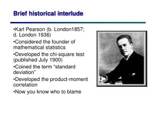
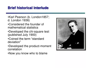
Brief historical interlude • Karl Pearson (b. London1857; d. London 1936) • Considered the founder of mathematical statistics • Developed the chi-square test (published July 1900) • Coined the term “standard deviation” • Developed the product-moment correlation • Now you know who to blame
Chi-square test of significance • Χ2 tests how cases are distributed across a variable • One variable—how its distribution compares to a • second, given distribution. • Two variables—tests whether the two variables are • related (statistically) to each other • Popular for crosstabs • H0: every i.v. category has the same distribution • across the d.v. as the total—i.e., the i.v. doesn’t • matter (the two variables are unrelated).
Chi-square (cont.) • The idea is that we calculate a statistic (i.e., we use a particular formula to calculate a number), where we know that the statistic has a certain distribution (in this case what’s called a chi-square distribution) that will occur simply by chance variation (in a sample). I.e., this statistic has a known (not normal) sampling distribution. • Because we know the distribution of this statistic, we can tell whether the result we get (the number that we calculate) is larger than one would expect by chance. • If it is, we conclude (in the case of two variables) that they are in fact related.
Here’s the formula: As you can see, once we figure out what frequencies we’re talking about, it’s not a very complicated formula. Nevertheless, SPSS will do the calculations for us. (SPSS is really good at multiplying, dividing, stuff like that.) Chi-square (cont.)
Here’s the distribution: Pearson’s great insight was to figure out that if there is in fact no relationship between two variables, if you draw repeated samples and calculate the formula on the last slide, you’ll get this kind of distribution simply because of chance variation. What we do in practice is to draw one sample and make the calculation. If the number we get is large enough, it tells us that we almost certainly didn’t get this number by chance. I.e., there really is a relation-ship between these variables in the population. Chi-square (cont.)
Chi-square (cont.) • The distribution is what you would expect by chance. It’s very likely you would get a small value and very unlikely that you would get larger and larger values. (The x-axis isn’t labeled, but distribution starts at zero.) • If you look back at the formula, you can see that the larger the difference between what you expected (given no relationship) and what you observed, the larger will be the chi-square number. • If it’s large enough, it tells you that you almost certainly didn’t get this number by chance. I.e., there really is a relationship between these variables in the population.
Example: Does an observed frequency distributionmatch the population distribution? • A study of grand juries in one county compared the demographic characteristics of jurors with the general population, to see if the jury panels were representative. The investigators wanted to know whether the jurors were selected at random from the population of this county. (This is an example of comparing one distribution with a second distribution. In this case, the second distribution is that of the population of the county on some characteristic.) • The observed data are given on the next page.
Example continued…. Observed data
Example continued…. Expected data
Example continued…. • As noted, the test statistic is: • Given our data,
The chi-square table • To use the table, we need what is called the degrees of freedom. • In this case, the degree of freedom is the number of categories minus 1, or 4-1=3. • Just like the t-table, we look up 3 on the table, and then look for the test statistic and report the bounds.
Example concluded • The df are (4-1)=3, and the p-value is therefore roughly 0. (Read values across the top as the area to the right of the critical value.) • So, with simple random sample, we conclude that it is almost impossible for a jury to differ this much from the county age distribution. The inference is that grand juries are not selected at random.
Now with a picture… • Chi-sq critical values • (area to the right of crit val.)
Testing independence with chi-square • In a certain town, there are about 1 million voters. An SRS of 10,000 was chosen to study the relationship between gender and participation. • Are gender and voting independent? • We can answer this with a chi-square test. • First, we need the expected values for each cell.
Expected values • The expected value for each cell is simply: • For men who voted, this is: • Thus, we have the following:
Observed and expected values We calculate the test statistic in the same way as before:
The test statistic The degrees of freedom are:
The p-value • The p-value is therefore around 1%. • Based on the p-value, we reject the null hypothesis and conclude that voting and gender are not independent. Or, in other words, men and women (in the population) don’t vote the same way.
Caveats, complications • Caveat: low frequencies can befuddle chi-square. When the expected frequency in a cell is below about 10, the values aren’t quite what they should be. • One “solution” is to recode categories so the expected frequencies aren’t so small. • There are some other “corrections” that one can make (but we won’t go into).
Testing caveat #1 • There is nothing special about 5% or 1%. • If our significance level is 5%, what is the difference between a p-value of 4.9% and a p-value of 5.1%? • One is statistically significant, and one is not. • But does that make sense? • One solution (not often used): report the p-value, not just the conclusion.
Testing caveat #2 • Data snooping • What does a significance level of 5% mean? • There is a 5% chance of rejecting the null hypothesis when it is actually true. • If our significance level is 5%, how many results would be “statistically significant” just by chance if we ran 100 tests? • We would expect 5 to be “statistically significant,” • and 1 to be “highly significant.”
Testing caveat #2 continued…. • So what can we do? • 1. One can state how many tests were run before statistically significant results turned up. • 2. If possible, one can test one’s conclusions on an independent set of data. • 3. Again, there are some statistical procedures that can help—basically playing off the idea that (at the 5% level) one should get 5% of the results significant merely by chance.
Testing caveat #3 • Was the result important? • What is the magnitude of the difference? In the example above, 65.3% of men voted, 62.8% of women voted). Chi-square doesn’t tell you that. • Even the level of significance doesn’t tell you that. (Yes, it’s related, but it depends on the number of cases, so you can’t simply say that a difference significant at, say, the 1% level is really big.) • This leads directly to the next topic: measures of assoc.
Testing caveat #3 conclusion • The moral of the story is: • A statistically significant difference may not be important. • And… • An important difference may not be statistically significant.