Download
1 / 36
370 likes | 571 Views
Probabilistic Context Free Grammars. Chris Brew. Ohio State University. Context Free Grammars. HMMs are sophisticated tools for language modelling based on finite state machines. This limits their descriptive power Context-free grammars go beyond FSMs

E N D
Probabilistic Context Free Grammars Chris Brew Ohio State University
Context Free Grammars • HMMs are sophisticated tools for language modelling based on finite state machines. • This limits their descriptive power • Context-free grammars go beyond FSMs • They can encode longer range dependencies than FSMs • They too can be made probabilistic
An example s -> np vp s -> np vp pp np -> det n np -> np pp vp -> v np pp -> p np n -> girl n -> boy n -> park n -> telescope v -> saw p -> with p -> in Sample sentence: “The boy saw the girl in the park with the telescope”
Multiple analyses • 2 of the 5 are
How serious is this ambiguity? • Very serious, ambiguities in different places multiply • Easy to get millions of analyses for simple seeming sentences • Maybe we can use probabilities to disambiguate, just as we chose from exponentially many paths through FSM • Fortunately, similar techniques apply
Probabilistic Context Free Grammars • Same as context free grammars, with one extension • Where there is a choice of productions for a non-terminal, give each alternative a probability. • For each choice point, sum of probabilities of available options is 1 • i.e. Production probability is p(rhs|lhs)
An example s -> np vp:0.8 s -> np vp pp:0.2 np -> det n:0.5 np -> np pp:0.5 vp -> v np:1.0 pp -> p np:1.0 n -> girl:0.25 n -> boy :0.25 n -> park:0.25 n -> telescope:0.25 v -> saw:1.0 p -> with:0.5 p -> in:0.5 Sample sentence: “The boy saw the girl in the park with the telescope”
The “low” attachment p(“np vp”|s) * p(“det n”|np) * p(“the”|det) * p(“boy”|n) * p(“v np”|vp) * p(“det n”|np) * p(“the”|det) * ...
The “high” attachment p(“np vp pp”|s) * p(“det n”|np) * p(“the”|det) * p(“boy”|n) * p(“v np”|vp) * p(“det n”|np) * p(“the”|det) * ... Note: I’m not claiming that this matches any particular set of psycholinguistic claims, only that the formalism allows such distinctions to be made.
Generating from Probabilistic Context Free Grammars • Start with the distinguished symbol “s” • Choose a way of expanding “s” • This introduces new non-terminals (eg. “np” “vp”) • Choose ways of expanding these • Carry on until no more non-terminals
Issues • The space of possible trees is infinite. • But the sum of probabilities for all trees is 1 • There is a strong assumption built in to the model • Expansion probability is independent of position of non-terminal within tree • This assumption is questionable.
Training for Probabilistic Context Free Grammars • Supervised: you have a treebank • Unsupervised: you have only words • In between: Pereira and Schabes
Supervised Training • Look at the trees in your corpus • Count the number of times each lhs -> rhs occurs • Divide these counts by number of times each lhs occurs • Maybe smooth as described in the lecture on probability estimation from counts
Unsupervised Training • These are Rabiner’s problems, but for PCFGs • Calculate the probability of a corpus given a model • Guess the sequence of states passed through • Adapt the model to the corpus
Hidden Trees • All you see is the output: • “The boy saw the girl in the park” • But you can’t tell which of several trees led to that sentence • Each tree may have a different probability. Although trees which use the same rules the same number of times must give the same answer. • Don’t know which state you are in.
The three problems • Probability estimation • Given a sequence of observations O and a grammar G. Find P(O|G) • Best tree estimation • Given a sequence of observations O and a grammar G, find a Tree which maximizes P(O,Tree|G).
The third problem • Training • Adjust the model parameters so that P(O|G) is as large as possible for given O. Hard problem because there are so many adjustable parameters which could vary. Worse than for HMMs. More local maxima.
Probability estimation • Easy in principle. Marginalize out the trees, leaving probability of strings. • But this involves sum over exponentially many trees. • Efficient algorithm keeps track of inside and outside probabilities.
Inside Probability • The probability that non-terminal NT expands to the words between i and j
Outside probability • Dual of inside probability. NP A MAN ... SENT A LETTER ... i j SENT A LETTER
Corpus probability • Inside probability of S node and entire string is probability of all ways of making sentences over that string • Product over all strings in corpus is corpus probability • Can also get corpus probability from outside probabilities
Training • Uses inside and outside probabilities • Starts from an initial guess • Improves the initial guess using data • Stops at a (locally) best model • Specialization of the EM algorithm
Expected rule counts • Consider p(uses rule lhs -> rhs to cover i through j) • Four things need to happen • Generate outside words leaving hole for lhs • Choose correct rhs • Generate word seen between i and k from first item in rhs (inside probability) • Generate words seen between k and j using other items in rhs (more inside probailities)
Refinements • In practice there are very many local maxima, so strategies which involve generating hundreds of thousands of rules may fail badly. • Pereira and Schabes discovered that letting the system know some limited stuff about bracketting is enough to guide it to correct answers • Different grammar formalisms (TAGs, Categorial Grammars...)
A basic parsing algorithm • The simplest statistical parsing algorithm is called CYK or CKY. • It is a statistical variant of a bottom-up tabular parsing algorithm that you should have seen in 684.01 • It (somewhat surprisingly) turns out to be closely related to the problem of multiplying matrices.
Basic CKY (review) • Assume we have organized the lexicon as a function lexicon: string -> nonterminal set • Organize these nonterminals into the relevant parts of a two dimensional array indexed by left and right end of the item For I = 1 to length(sentence) dochart[I,I+1] = lexicon(sentence[i]) endfor
Basic CKY • Assume we have organized the grammar as a function grammar: nonterminal -> nonterminal -> nonterminal set
Basic CKY • Build up new entries from existing entries, working from shorter entries to longer ones for l = 2 to length(sentence) do // l is length of constituent for s = 1 to len – l + 1 do // s is start of rhs1 for t = 1 to l-1 do (left,mid,right) = (s,s+t,s+l) chart[left,right] = combine(chart[left,mid],chart[mid,right]) endfor endfor endfor
Basic CKY • Combine is fun combine(set1,set2) result = empty for item1 in set1 do for item2 in set2 do result = union result (grammar item1 item2) endfor endfor return result
Going statistical • The basic algorithm tracks labels for each substring of the input • The cell contents are sets of labels • A statistical version keeps track of labels and their probabilities • Now the cell contents must be weighted sets
Going statistical • Make the grammar and lexicon produce weighted sets. gexicon: word -> real*nt set grammar: real*nt->real*nt -> real*nt set • We now need an operation corresponding to set union for weighted sets. • {s:0.1,np:0.2} WU {s:0.2,np:0.1} = ???
Going statistical (one way) {s:0.1,np:0.2} WU {s:0.2,np:0.1} = {s:0.3,np:0.3} If we implement this, we get a parser that calculates the inside probability for each label on each span.
Going statistical (another way) {s:0.1,np:0.2} WU {s:0.2,np:0.1} = {s:0.2,np:0.2} If we implement this, we get a parser that calculates the best parse probability for each label on each span. The difference is that in one case we are combining weights with +, while in the second we use max
Building trees • Make the cell contents be sets of trees • Make the lexicon be a function from words to little trees • Make the grammar be a function from pairs of trees to sets of newly created (bigger) trees • Set union is now over sets of trees • Nothing else needs to change
Building weighted trees • Make the cell contents be sets of trees, labelled with probabilities • Make the lexicon be a function from words to weighted (little trees) • Make the grammar be a function from pairs of weighted trees to sets of newly created (bigger) trees • Set union is now over sets of weighted trees • Again we have a choice of min or +, to get either parse forest or just best parse
Where to get more information • Manning and Schütze chapter 11 • Charniak chapters 5 and 6 • AllenNatural Language Understandingch 7 • Lisp code associated with Natural Language Understanding • Goodman: Semiring parsing (http://www.aclweb.org/anthology/J99-1004)