Download
1 / 5
50 likes | 157 Views
Inventory Theory Continuous Review Math 305. 12/7/08. Continuous Review. Previous model: periodic review orders placed at the begining of periods Continuous review: an order may be placed at any time What is an inventory policy? when to order more how much to order Costs

E N D
Continuous Review Previous model: periodic review • orders placed at the begining of periods Continuous review: an order may be placed at any time What is an inventory policy? • when to order more • how much to order Costs • ordering /production (paperwork, delivery charges, per unit charges) • holding (storage, spoilage, opportunity • shortage (possible loss of sale, cost of filling back order) • revenues (not usually counted) • salvage value (at end of inventory period)
Deterministic Example, No Shortages My factory needs 8000 speakers/month for the TVs it makes • speakers are produced in batches • setup cost per batch: $12,000 per run (retooling, startup,...) • per speaker cost of $10 How much do I produce/order at a time? (Q) Q (speakers) Q/a (time) In general K = set up cost c = per unit cost → production cost/cycle = K + cQ a = rate of demand → cycle length = Q/a h = holding cost → holding cost per cycle = (Q/a)(Q/a) h = (hQ2)/2a
No Shortages Total cost per cycle = K + cQ + (hQ2)/2a Cost per unit time T(Q) = K + cQ + (hQ2)/2a = aK/Q + ac + hQ/2 Q/a T(Q) dT/dQ = -aK/Q2 +h/2 Q* = √2aK/h = EOQ t = Q/a = √ 2K/ah Q* Q TVs: T(Q) = (8000)(12,000)/Q + 8000 + .30Q/2 Q* = 25,298 t* = 3.2 months
Shortages Allowed Shortage cost p per unfilled unit of demand per unit time S Q S/a Q/a shortage: p(Q/a-S/a)(Q-s)/2 = p(Q-S)2 /2a T(Q,S) = K + cQ - hS2/2a + p(Q-S)2/2a = aK/Q + ac + hS2/2Q + p(Q-S) 2/2a Q/a (... messy partial derivatives...) S* = √2aK/h √ p/(p+h) Q* = √2aK/h √(p+h)/p What happens as p → ∞? as p↓ P for speakers = 1.10 S* = EOQ(√ 1.1/(1.1+.3) = 22,424 Q* = EOQ(√ (1.1+.3)/1.1) = 28,540 Q-S = max shortage = 6116