Download
1 / 30
300 likes | 376 Views
Learn about strategies to dramatically reduce the number of data points needed in signal processing, using methods such as Discrete Fourier Transform and ideal filter/error function filter. Explore Nyquist Theorem, convolution, and frequency-time techniques with practical examples and applications. Discover how the error function filter can optimize data reduction, and the importance of understanding pulsar numbers. Gain insights into filtering techniques, convolution ranges, and oscillation utilization for efficient processing and analysis.

E N D
Error Function FilterRobert L. ColdwellUniversity of FloridaLSC August 2005 LIGO-G050352-00-Z Reducing the number of data points
Introduction • Discrete Fourier Transform Definitions • The Nyquist Theorem • Ideal Filter/Error Function Filter • Pulsar numbers • Dramatically reducing the number of needed data points
Convolution Frequency Time
Nyquist Theorem1 Define 1 Loosely based on Alan V. Oppenheimer, Ronald W. Schafer with John R. Buck,Discrete-time Signal Processing – Prentice Hall Signal Processing Series – Alan V. Oppenheimer, editor, Second edition 1999 – first 1989
Note upper limit of N/2-1 This sum is N for m=kN, zero otherwise The function s(t)
Inserting S(f) Dsamp is periodic by construction Nyquist theorem in frequency
Back Transform • The back transform over all N points is not wanted since it will produce the spiky function transformed forward. • Define an ideal filter as
The sum is over M as in N=MN With appropriate restrictions But in any case define This form is a setup for convolution
Using the convolution theorem The time tm is any time, the time tk is for a data point. This is where the dramatic reduction in data points needed takes place. The Nyquist Theorem in time
Ideal Filter/Error Function Filter H is not required to extend from -1/2t to 1/2t The ideal f0 to f1 filter
Ideal filter transformation The fact that this sum is to N includes the extra point at N/2 The extra term ↑ Subrtacting ½ the first term ↑ A few steps are skipped involving 1/(1-exp(-j21/T)). All steps are rigorous for the sums
Ideal h(t,f0,f1) The second term as T
Error function filter Let x=(f-f0)/w, then for f<f0 Equivalent erfs allow overlapping regions to exactly sum to 1 And for f > f0
Herrf(f,f0,f1) The f0 = 59 Hz, f1=61 Hz w = 0.125 Hz.
Error function filter/ ideal filter f = 1/7 sec. w=f
herrf(t,f0,f1,w) Approximation of the integral result requires integration by parts In a reversal of the Nyquist theorem, the correctly periodic version is The exp(-(wt)2) term makes the sum rapidly convergent This now differs from the ideal filter only by the exponential factor.
Limiting the convolution range For |t-tk| > 6/(w), the exponential part of h(t,f0,f1,w) is less then This leads to a definition kmin(t)=(t-6/(w))/t such that Even for infinite T, this sum is finite. For t such that kmin(t) > -N/2 and kmax(t)<N/2 dH(t) does not depend on T
|h(t,f0,f1,w)| Time in seconds.
h(t,f0,f1,w) The oscillations can be used to shift the frequency. Note that h can be calculated once, then shifted and re-used over and over, the sine and cosines need not be recalculated. Convolution reduces to a single set of multiplications and sums for each output data point. Small region of time showing the oscillations in real and imaginary h(t)
Second region The convolution with h(t,f1,f2,w) produces complex data. The imaginary part is shown above.
Second region in frequency Real part of transform of convoluted data between 32/Time and 50/time using 50-32+10 data points
Second region in frequency Ignoring the 10, the data reduction factor is Real part of transform of convoluted data between 32/Time and 50/time using 50-32+10 data points
Pulsar numbers The size of F was found by Cornish and Larson to be ~ 0.01 Hz[i], Thus there needs to be an output point every 10 seconds to follow the Doppler motion of B0531+21 which has a quadrupole frequency of 59.620.01 Hz. [i] Neil J. Cornish and Shane L. Larson, “LISA data analysis: Doppler demodulation”, Class. Quantum Grav. 20 (2003) S163-S170 – online at stacks.iop.org/CQG/20/S163 Data reduction factor ~ 16384/0.02 = 819200
|h(t)| for 0.02 width signal The time range on this plot is from –500 seconds to + 500 seconds.
Omissions The phase will need to be monitored, if it drifts the signal will cancel to zero. – possibly the violin modes will help. If the convolution went straight from the input data, noise in the region would in principle rise as T1/2 while the signal would rise as T. The noise is systematic and has many properties that identify it, an intermediate step in which known sources of frequencies that overlap the pulsar frequency are examined and removed will be investigated.