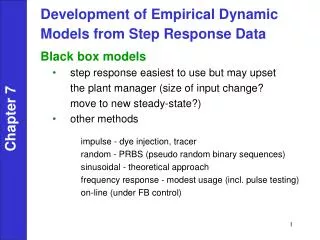
Development of Empirical Dynamic Models from Step Response Data Black box models

1. Development of Empirical Dynamic • Models from Step Response Data • Black box models • step response easiest to use but may upset the plant manager (size of input change? move to new steady-state?) • other methods Chapter 7 • impulse - dye injection, tracer • random - PRBS (pseudo random binary sequences) • sinusoidal - theoretical approach • frequency response - modest usage (incl. pulse testing) • on-line (under FB control)

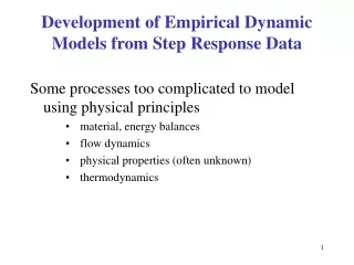
2. Some processes too complicated to model using • physical principles • material, energy balances • flow dynamics • physical properties (often unknown) • thermodynamics • Example 1: distillation column • 50 plates • For a 50 plate column, dynamic models have • many ODEs that require model simplification; and physical properties must be known; e.g., HYSYS • black box models (only good for fixed operating conditions) but requires operating plant (actual data) • theoretical models must be used prior to • plant construction or for new process chemistry Chapter 7

3. Chapter 7 • Need to minimize disturbances during a plant test

4. Simple Process Models 1st order system with gain K, dead time  and time constant ; 3 parameters to be fitted. Step response: Chapter 7

5. For a 1st order model, we note the following characteristics (step response) (1) The response attains 63.2% of its final response at one time constant (t =  ). (2) The line drawn tangent to the response at maximum slope (t = ) intersects the 100% line at (t =  ). [see Fig. 7.2] Chapter 7 K is foundfrom the steady state response for an input change magnitude M. • There are 4 generally accepted graphical techniques • for determining first order system parameters , : • 63.2% response • point of inflection • S&K method • semilog plot

6. Chapter 7 (θ = 0)

7. Chapter 7 Inflection point hard to find with noisy data.

8. S & K Method for Fitting FOPTD Model • Normalize step response (t = 0, y = 0; t →∞, y = 1) • Use 35 and 85% response times (t1 and t2) q = 1.3 t1 – 0.29 t2 t = 0.67 (t2 – t1) (based on analyzing many step responses) K found from steady state response • Alternatively, use Excel Solver to fit q and t using y (t) = K [1 – e –(t-q)/τ] and data of y vs. t Chapter 7

9. Fitting an Integrator Model to Step Response Data In Chapter 5 we considered the response of a first-order process to a step change in input of magnitude M: Chapter 7 For short times, t < t, the exponential term can be approximated by so that the approximate response is: (straight line with slope of y1(t=0))

10. is virtually indistinguishable from the step response of the integrating element In the time domain, the step response of an integrator is Chapter 7 Comparing with(7-22), matches the early ramp-like response to a step change in input.

11. Chapter 7 Figure 7.10. Comparison of step responses for a FOPTD model (solid line) and the approximate integrator plus time delay model (dashed line).

12. Chapter 7

13. Chapter 5

14. Chapter 7

15. Chapter 7

16. Smith’s Method 20% response: t20 = 1.85 60% response: t60 = 5.0 t20 / t60 = 0.37 from graph Chapter 7 Solving,

17. Using Excel Solver to Fit Transfer Function Models • use y (data) vs. y (predicted) • column 1 is data (taken at different times), or y1 • column 2 is model prediction (same time values as above), or y2 • target cell is S (y1 - y2)2 , to be minimized • specify parameters to be changed in reference cells (e.g. t1 = 1, t2 = 2) • open solver dialog box to check settings • click on < solve > (calls optimization program) Chapter 7

18. Chapter 7

19. Chapter 7

20. Chapter 7

21. Chapter 7 Previous chapter Next chapter