Download
1 / 17
180 likes | 369 Views
Explore the delocalized approach to bonding through Molecular Orbital Theory, understanding MO formation for diatomic molecules like H2, energy ordering of MOs, and the significance of in-phase and out-of-phase overlap.

E N D
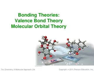
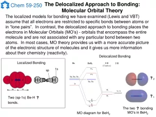
The Delocalized Approach to Bonding: Molecular Orbital Theory The localized models for bonding we have examined (Lewis and VBT) assume that all electrons are restricted to specific bonds between atoms or in “lone pairs”. In contrast, the delocalized approach to bonding places the electrons in Molecular Orbitals (MO’s) - orbitals that encompass the entire molecule and are not associated with any particular bond between two atoms. In most cases, MO theory provides us with a more accurate picture of the electronic structure of molecules and it gives us more information about their chemistry (reactivity). Delocalized Bonding Localized Bonding 1s sp 2 1 Two (sp-1s) Be-H bonds. The two bonding MO’s in BeH2 MO diagram for BeH2
Molecular Orbital Theory Molecular orbitals are constructed from the available atomic orbitals in a molecule. This is done in a manner similar to the way we made hybrid orbitals from atomic orbitals in VBT. That is, we will make the MO’s for a molecule from Linear Combinations of Atomic Orbitals (LCAO). In contrast to VBT, in MO theory the atomic orbitals will come from several or all of the atoms in the molecule. Once we have constructed the MO’s, we can build an MO diagram (an energy level diagram) for the molecule and fill the MO’s with electrons using the Aufbau principle. Some basic rules for making MO’s using the LCAO method: 1) n atomic orbitals must produce n molecular orbitals (e.g. 8 AO’s must produce 8 MO’s). 2) To combine, the atomic orbitals must be of the appropriate symmetry. 3) To combine, the atomic orbitals must be of similar energy. 4) Each MO must be normal and must be orthogonal to every other MO. + + 1 Be 2s H 1s H 1s
Molecular Orbital Theory Diatomic molecules: The bonding in H2 Each H atom has only a 1s orbital, so to obtain MO’s for the H2 molecule, we must make linear combinations of these two 1s orbitals. Consider the addition of the two 1s functions (with the same phase): This produces an MO around both H atoms and has the same phase everywhere and is symmetrical about the H-H axis. This is known as a bonding MO and is given the label g because of its symmetry. + 1sA 1sB g = 0.5 (1sA + 1sB) Consider the subtraction of the two 1s functions (with the same phase): This produces an MO over the molecule with a node between the atoms (it is also symmetrical about the H-H axis). This is known as an antibonding MO and is given the label u* because of its symmetry. The star indicates antibonding. - 1sA 1sB u* = 0.5 (1sA - 1sB) - + Remember that: is equivalent to:
Molecular Orbital Theory Diatomic molecules: The bonding in H2 You may ask … Why is g called “bonding” and u* “antibonding”? What does this mean? How do you know the relative energy ordering of these MO’s? Remember that each 1s orbital is an atomic wavefunction (1s) and each MO is also a wave function, , so we can also write LCAO’s like this: u* = 2 = 0.5 (1sA - 1sB) g = 1 = 0.5 (1sA + 1sB) Remember that the square of a wavefunction gives us a probability density function, so the density functions for each MO are: (1)2 = 0.5 [(1sA 1sA) + 2(1sA 1sB) +(1sB 1sB)] and (2)2 = 0.5 [(1sA 1sA) - 2(1sA 1sB) +(1sB 1sB)] The only difference between the two probablility functions is in the cross term (in bold), which is attributable to the kind and amount of overlap between the two 1s atomic wavefunctions (the integral (1sA 1sB) is known as the “overlap integral”, S). In-phase overlap makes bonding orbitals and out-of-phase overlap makes antibonding orbitals…why?
Molecular Orbital Theory Diatomic molecules: The bonding in H2 Consider the electron density between the two nuclei: the red curve is the probability density for HA by itself, the blue curve is for HB by itself and the brown curve is the density you would get for 1sA + 1sB without any overlap: it is just (1sA)2 + (1sB)2 {the factor of ½ is to put it on the same scale as the normalized functions}. The function (1)2 is shown in green and has an extra + 2 (1sA 1sB) of electron density than the situation where overlap is neglected. The function (2)2 is shown in pink and has less electron density between the nuclei {- 2(1sA 1sB)} than the situation where overlap is neglected. (1)2 = 0.5 [(1sA 1sA) + 2(1sA 1sB) +(1sB 1sB)] (2)2 = 0.5 [(1sA 1sA) - 2(1sA 1sB) +(1sB 1sB)] The increase of electron density between the nuclei from the in-phase overlap reduces the amount of repulsion between the positive charges. This means that a bonding MO will be lower in energy (more stable) than the corresponding antibonding MO or two non-bonded H atoms.
Molecular Orbital Theory Diatomic molecules: The bonding in H2 So now that we know that the bonding MO is more stable than the atoms by themselves and the u* antibonding MO, we can construct the MO diagram. H H2 H To clearly identify the symmetry of the different MO’s, we add the appropriate subscripts g (symmetric with respect to the inversion center) and u (anti-symmetric with respect to the inversion center) to the labels of each MO. The electrons are then added to the MO diagram using the Aufbau principle. u* Energy 1s 1s g Note: The amount of stabilization of the g MO (indicated by the red arrow) is slightly less than the amount of destabilization of the u* MO (indicated by the blue arrow) because of the pairing of the electrons. For H2, the stabilization energy is 432 kJ/mol and the bond order is 1.
Molecular Orbital Theory Diatomic molecules: The bonding in He2 He also has only 1s AO, so the MO diagram for the molecule He2 can be formed in an identical way, except that there are two electrons in the 1s AO on He. The bond order in He2 is (2-2)/2 = 0, so the molecule will not exist. However the cation [He2]+, in which one of the electrons in the u* MO is removed, would have a bond order of (2-1)/2 = ½, so such a cation might be predicted to exist. The electron configuration for this cation can be written in the same way as we write those for atoms except with the MO labels replacing the AO labels: [He2]+ = g2u1 He He2 He u* Energy 1s 1s g Molecular Orbital theory is powerful because it allows us to predict whether molecules should exist or not and it gives us a clear picture of the of the electronic structure of any hypothetical molecule that we can imagine.
Molecular Orbital Theory Diatomic molecules: Homonuclear Molecules of the Second Period Li has both 1s and 2s AO’s, so the MO diagram for the molecule Li2 can be formed in a similar way to the ones for H2 and He2. The 2s AO’s are not close enough in energy to interact with the 1s orbitals, so each set can be considered independently. Li Li2 Li 2u* The bond order in Li2 is (4-2)/2 = 1, so the molecule could exists. In fact, a bond energy of 105 kJ/mol has been measured for this molecule. Notice that now the labels for the MO’s have numbers in front of them - this is to differentiate between the molecular orbitals that have the same symmetry. 2s 2s 2g Energy 1u* 1s 1s 1g
Molecular Orbital Theory Diatomic molecules: Homonuclear Molecules of the Second Period Be also has both 1s and 2s AO’s, so the MO’s for the MO diagram of Be2 are identical to those of Li2. As in the case of He2, the electrons from Be fill all of the bonding and antibonding MO’s so the molecule will not exist. Be Be2 Be The bond order in Be2 is (4-4)/2 = 0, so the molecule can not exist. Note: The shells below the valence shell will always contain an equal number of bonding and antibonding MO’s so you only have to consider the MO’s formed by the valence orbitals when you want to determine the bond order in a molecule! 2u* 2s 2s 2g Energy 1u* 1s 1s 1g
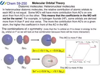
Molecular Orbital Theory Diatomic molecules: The bonding in F2 Each F atom has 2s and 2p valence orbitals, so to obtain MO’s for the F2 molecule, we must make linear combinations of each appropriate set of orbitals. In addition to the combinations of ns AO’s that we’ve already seen, there are now combinations of np AO’s that must be considered. The allowed combinations can result in the formation of either or type bonds. The combinations of symmetry: This produces an MO over the molecule with a node between the F atoms. This is thus an antibonding MO of u symmetry. + 2pzA 2pzB u* = 0.5 (2pzA + 2pzB) This produces an MO around both F atoms and has the same phase everywhere and is symmetrical about the F-F axis. This is thus a bonding MO of g symmetry. - 2pzA 2pzB g = 0.5 (2pzA - 2pzB)
Molecular Orbital Theory Diatomic molecules: The bonding in F2 The first set of combinations of symmetry: This produces an MO over the molecule with a node on the bond between the F atoms. This is thus a bonding MO of u symmetry. + 2pyA 2pyB u = 0.5 (2pyA + 2pyB) This produces an MO around both F atoms that has two nodes: one on the bond axis and one perpendicular to the bond. This is thus an antibonding MO of g symmetry. - 2pyA 2pyB g* = 0.5 (2pyA - 2pyB)
Molecular Orbital Theory Diatomic molecules: The bonding in F2 The second set of combinations with symmetry (orthogonal to the first set): This produces an MO over the molecule with a node on the bond between the F atoms. This is thus a bonding MO of u symmetry. + 2pxA 2pxB u = 0.5 (2pxA + 2pxB) This produces an MO around both F atoms that has two nodes: one on the bond axis and one perpendicular to the bond. This is thus an antibonding MO of g symmetry. - 2pxA 2pxB g* = 0.5 (2pxA - 2pxB)
You will typically see the diagrams drawn in this way. The diagram is only showing the MO’s derived from the valence electrons because the pair of MO’s from the 1s orbitals are much lower in energy and can be ignored. Although the atomic 2p orbitals are drawn like this: they are actually all the same energy and could be drawn like this: at least for two non-interacting F atoms. Notice that there is no mixing of AO’s of the same symmetry from a single F atom because there is a sufficient difference in energy between the 2s and 2p orbitals in F. Also notice that the more nodes an orbital of a given symmetry has, the higher the energy. Note: The the sake of simplicity, electrons are not shown in the atomic orbitals. Molecular Orbital Theory MO diagram for F2 F F F2 3u* 1g* 2p (px,py) pz 2p 1u Energy 3g 2u* 2s 2s 2g
Molecular Orbital Theory MO diagram for F2 F F F2 Another key feature of such diagrams is that the -type MO’s formed by the combinations of the px and py orbitals make degenerate sets (i.e. they are identical in energy). The highest occupied molecular orbitals (HOMOs) are the 1g* pair - these correspond to some of the “lone pair” orbitals in the molecule and this is where F2 will react as an electron donor. The lowest unoccupied molecular orbital (LUMO) is the 3u* orbital - this is where F2 will react as an electron acceptor. 3u* LUMO 1g* HOMO 2p (px,py) pz 2p 1u Energy 3g 2u* 2s 2s 2g
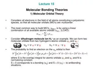
Molecular Orbital Theory MO diagram for B2 In the MO diagram for B2, there several differences from that of F2. Most importantly, the ordering of the orbitals is changed because of mixing between the 2s and 2pz orbitals. From Quantum mechanics: the closer in energy a given set of orbitals of the same symmetry, the larger the amount of mixing that will happen between them. This mixing changes the energies of the MO’s that are produced. The highest occupied molecular orbitals (HOMOs) are the 1u pair. Because the pair of orbitals is degenerate and there are only two electrons to fill, them, each MO is filled by only one electron - remember Hund’s rule. Sometimes orbitals that are only half-filled are called “singly-occupied molecular orbtials” (SOMOs). Since there are two unpaired electrons, B2 is a paramagnetic (triplet) molecule. B B B2 3u* 1g* 2p (px,py) pz 2p 3g LUMO Energy HOMO 1u 2u* 2s 2s 2g
2s-2pz mixing Molecular Orbital Theory Diatomic molecules: MO diagrams for Li2 to F2 Remember that the separation between the ns and np orbitals increases with increasing atomic number. This means that as we go across the 2nd row of the periodic table, the amount of mixing decreases until there is no longer enough mixing to affect the ordering; this happens at O2. At O2 the ordering of the 3g and the 1u MO’s changes. As we go to increasing atomic number, the effective nuclear charge (and electronegativity) of the atoms increases. This is why the energies of the analogous orbitals decrease from Li2 to F2. The trends in bond lengths and energies can be understood from the size of each atom, the bond order and by examining the orbitals that are filled. In this diagram, the labels are for the valence shell only - they ignore the 1s shell. They should really start at 2g and 2u*.
UV-PES spectrum of N2 I = h - KE = 21.1 eV - KE ejected photoelectron UV photon ionized molecule Molecular Orbital Theory Ultra-Violet Photoelectron Spectroscopy (UV-PES) The actual energy levels of the MO’s in molecules can be determined experimentally by a technique called photoelectron spectroscopy. Such experiments show that the MO approach to the bonding in molecules provides an excellent description of their electronic structure. In the UV-PES experiment, a molecule is bombarded with high energy ultraviolet photons (usually Ephoton = h = 21.1 eV). When the photon hits an electron in the molecule it transfers all the energy to the electron. Part of the energy (equal to the ionization potential, I, of the MO in which the electron was located) of the photoelectron is used to leave the molecule and the rest is left as kinetic energy (KE). The kinetic energy of the electrons are measured so I can be calculated from the equation: The shape and number of the peaks provides other information about the type of orbital the photoelectron came from. We will not worry about the details, but you can find out more about this in a course on spectroscopy.