Download
1 / 41
410 likes | 513 Views
Learn about scaling techniques for managing vast geospatial data in databases. Explore strategies for spatial search queries and database enhancements.

E N D
Efficient search indices for geospatial data in a relational database Gyorgy (George) Fekete Dept. Physics and Astronomy Johns Hopkins University
Acknowledgements • Alex Szalay • NVO, SDSS, iVDGL, ... • Jim Gray • Databases, SQL Server • Ani Thakar, Tamas Budavari • SDSS pipeline, Geometric libraries
Motivation • Growth of volume of data • terabytes per day • Increasing importance of databases in managing science data • Data mining : potential for new discoveries • Cross matching between multiple surveys • Much of this data is distributed on a sphere • astronomy and earth science • great interest in a universal, computer-friendly index on the sphere
Astronomy Data • “old days” • astronomers took photos. • Since the 1960’s • they began to digitize.New instruments are digital (100s of GB/nite)Detectors are following Moore’s law.Data avalanche: double every 2 years
Astronomy Data • Astronomers have a few Petabytes now. • Data volume and ownership • doubles every 2 years. • Data is public after 2 years. • So, 50% of the data is public. • Some have private access to 5% more data. • But….. • How do I get at that 50% of the data?
New Astronomy • Data “Avalanche” • the flood of Terabytes of data • present techniques of handling these data do not scale well with data volume • Systematic data exploration • will have a central role • statistical analysis of the “typical” objects • automated search for the “rare” events • Digital archives of the sky • will be the main access to data
Data Intensive Science • Data avalanche in astronomy and other sciences • old file-based solutions do not cut it • old data silos don’t work • old programming models don’t work • We have some new tricks! • Astronomy and Earth-Science • methods presented here deal with the topology and the geometry of the sphere
One Of These Tricks: • Map regions of the sphere to unique identifiers that can be used as references to those areas • elementary spherical geometry to identify a region • multi-resolution • compactly describe areas at arbitrary granularity
Support Spatial Searches Typical queries • What is near this point? • What objects are in this area? • What areas overlap this area?
Design Considerations • Has to • work with a relational database • represent areas of interest precisely • be scalable • be coordinate system neutral • maintain consistency with the topology of the sphere • Approach: • precise mathematical description of regions • methods for covering a region with an optimal set of discrete descriptors (trixels) • covermap of trixels used for accelarated query
Components • Region descriptions (continuous part) • region, convex, halfspace • API and a text language to describe • XML for inter-service, inter-application object transfer • Hierachical Triangular Mesh (discrete part) • trixels • covermaps • Database • extend the DB server engine with spatial access methods • implementing coarse filtering with table valued functions
Region is the union of convexes Convex is intersection of halfspaces Halfspace simple search cone circle Continuous Part: A Region
Disk, Circle, Search cone, ... Spherical Polygon yes, it is actually a convex (adj.) convex (n.) Band Lat/Lon (or Ra/Dec) rectangle anything else... Examples of Convexes
Halfspace Cutting plane makes two halfspaces Oriented plane makes one well defined halfspace
Halfspace D = cos (cone halfangle) h = (x, y, z, D) Completely defined by (directed) plane normal and distance along the normal
Point Inclusion In Region (x,y,z) P h = (x, y, z, D) Q P . (x, y, z) > D Point is inside a convex if and ony ifit is inside all halfspaces Point is inside a region if and ony ifit is inside at least one convex Q . (x, y, z) < D
Intersecting halfspaces can produce multiple connected components Anything you can think of can be expressed as a union of convexes Disconnected Components
Triangle Subdivision Scheme Each trixel can be named: eg S123222102 HTMId: depth limited trixels are represented 64-bit integers
HTMId Coherence level 3 level 4 level 5 1023 4092 - 4095 16368 - 16383 level 20 17575006175232 - 17592186044415
covermap is a set of trixels that cover a region Covermap Of Circle
Covermap Of California 15277198671872 - 1527827241369515298673508352 - 1530082099199915301089427456 - 15302968475647 ... ...15384572854272 - 15384841289727 44 trixels, but only 13 ranges Use covermaps and HtmIDs to coarse filter...
Database Part • From table of objects, consider only those whose key values are in the covermap • Of those that passed, perform calculation to complete query • Return result in table
Coarse and Fine Filtering In Queries use precise calculations use covermaps
Usage of Tables and Index Keys Create a function that generates keys that cluster related data together • if objects A and B are nearby, then the keys for A and B should be also be nearby in the Index space • HtmID Create a table-valued function that returns • list of key ranges (the covermap) containing all the pertinent values • covermap
Caveats • You cannot always get every key to be near all its neighbors • keys are sorted in one dimension • relatives are near in two-dimensional space • But we can come close • The ratio of false-positives to correct answers is a measure of how well you are doing. .
USGS Dataset Experiment 18,000 stream gauges 23,000 places
Sample Covermap select * from fHtmCoverCircleLatLon(39.3,-76.6, 100) HtmIDStart HtmIDEnd ---------------- ---------------- 14023336656896 14024141963263 14024410398720 14025215705087 14025484140544 14027363188735
Places Within 100 Miles Of Baltimore select ObjID from SpatialIndex join fHtmCoverCircleLatLon(39.3,-76.6, 100) On HtmID between HtmIDStart and HtmIDEndwhere Type = 'P' and dbo.fDistanceLatLon(39.3,-76.6, Lat, Lon) < 100 go Number of rows in cover join (coarse filter) 2223 Number of rows that are within 100 n. miles (after the fine filter). 1122 Number of places in DB 22993Time with covermap 35 Time without covermap 100
California As A Region declare @californiaRegion varchar(max) set @californiaRegion = 'REGION ' + 'rect latlon 39 -125' -- nortwest corner + '42 -120 ' -- center of Lake Tahoe + 'chull latlon 39 -124 ' -- Pt. Arena + '39 -120 ' -- Lake tahoe. + '35 -114.6 ' -- start Colorado River + '34.3 -114.1 ' -- Lake Havasu + '32.74 -114.5 ' -- Yuma + '32.53 -117.1 ' -- San Diego + '33.2 -119.5 ' -- San Nicholas Is + '34 -120.5 ' -- San Miguel Is. + '34.57 -120.65 ' -- Pt. Arguelo + '36.3 -121.9 ' -- Pt. Sur + '36.6 -122.0 ' -- Monterey + '38 -123.03 ' -- Pt. Rayes
California Cities select PlaceName from Place where HtmID in (select distinct SI.objID from fHtmCoverRegion(@californiaRegion) loop join SpatialIndex SIon SI.HtmID between HtmIdStart and HtmIdEnd and SI.type = 'P' join place P on SI.objID = P.HtmID cross join fHtmRegionToTable(@californiaRegion) Poly group by SI.objID, Poly.convexID having min(SI.x*Poly.x + SI.y*Poly.y + SI.z*Poly.z - Poly.d) >= 0) OPTION( FORCE ORDER) See Point Inclusion This is a popular query, so we can include it as a stored procedure
Point Inclusion With SQL (x,y,z) P h = (x, y, z, D) P . (x, y, z) > D P . (x, y, z) - D > 0 min(SI.x*Poly.x + SI.y*Poly.y +SI.z*Poly.z - Poly.d) >= 0)
Covermap Of California 15277198671872 - 1527827241369515298673508352 - 1530082099199915301089427456 - 15302968475647 ... ...15384572854272 - 15384841289727 44 trixels, but only 13 ranges Use covermaps and HtmIDs to coarse filter...
DB Function For Region Search select PlaceName from Place where HtmID in (select ObjID from fHtmRegionObjects(@californiaRegion,'P') ) Number of rows in cover join (coarse filter) 981 Number of rows that are within region 885 Number of places in DB 22993Time with covermap 110 Time without covermap 1210
SDSS • Digital map in 5 spectral bands covering ¼ of the sky. • Will obtain 40 TB of raw pixel data. • Photometric catalog with more than 200 million objects. • Spectra of ~ 1 million objects. • Data Release 3 – DR3: 150 M images, 480 k spectra.
Ambitious Survey • Info content > US Library of Congress • Before SDSS:total number of galaxies with measured parameters ~ 100k • After SDSS, we will have detailed parameters forover 100 Million galaxies!!
SDSS Processing Pipeline • Processed data ingested into a relational DBMS • Allows fast exploration and analysis - Data Mining • Heavily indexed to speed up access – HTM + DB Indices • Short queries can run interactively. • Long queries (> 1 hr) require a custom Batch Query System.
SDSS Data Access • Data Archive Server (DAS) • FITS files (raw data) • Images, spectra, corrected frames, atlas images, binned images, masks • Online form-based access at www.sdss.org • Rsync and wget file retrieval • Catalog Archive Server (CAS) • Science parameters extracted to catalogs • Stuffed into relational DBMS (SQL Server) • Online access via SkyServer at http://cas.sdss.org/, http://skyserver.sdss.org
Conclusion • HTM methods provide means for implementing ways to filter data so that expensive geometrical computations to satisfy a query are performed on only a small subset of the original data • The HTM is on its way to become one of the de facto standards for representing spatial information in astronomical catalogs, especially for large-scale surveys.