Download
1 / 55
550 likes | 751 Views
Lecture 8 CS157B. Decision Trees and Association Rules. Prof. Sin-Min Lee Department of Computer Science. Data Mining: A KDD Process. Knowledge. Pattern Evaluation. Data mining: the core of knowledge discovery process. Data Mining. Task-relevant Data. Selection. Data Warehouse.

E N D
Lecture 8 CS157B Decision Trees and Association Rules Prof. Sin-Min Lee Department of Computer Science
Data Mining: A KDD Process Knowledge Pattern Evaluation • Data mining: the core of knowledge discovery process. Data Mining Task-relevant Data Selection Data Warehouse Data Cleaning Data Integration Databases
Decision Trees • A decision tree is a special case of a state-space graph. • It is a rooted tree in which each internal node corresponds to a decision, with a subtree at these nodes for each possible outcome of the decision. • Decision trees can be used to model problems in which a series of decisions leads to a solution. • The possible solutions of the problem correspond to the paths from the root to the leaves of the decision tree.
Decision Trees • x • x • x • x • x • x • x • x • x • x • x • x • Q • Q • x • x • x • x • x • x • x • x • x • x • x • x • x • x • x • Example: The n-queens problem • How can we place n queens on an nn chessboard so that no two queens can capture each other? A queen can move any number of squares horizontally, vertically, and diagonally. Here, the possible target squares of the queen Q are marked with an x.
Let us consider the 4-queens problem. • Question: How many possible configurations of 44 chessboards containing 4 queens are there? • Answer: There are 16!/(12!4!) = (13141516)/(234) = 13754 = 1820 possible configurations. • Shall we simply try them out one by one until we encounter a solution? • No, it is generally useful to think about a search problem more carefully and discover constraints on the problem’s solutions. • Such constraints can dramatically reduce the size of the relevant state space.
Obviously, in any solution of the n-queens problem, there must be exactly one queen in each column of the board. Otherwise, the two queens in the same column could capture each other. Therefore, we can describe the solution of this problem as a sequence of n decisions: Decision 1: Place a queen in the first column. Decision 2: Place a queen in the second column. ...Decision n: Place a queen in the n-th column.
Backtracking in Decision Trees • Q • Q • Q • Q • Q • Q • Q • Q • Q • Q • Q • Q • Q • Q • Q • Q • Q • Q empty board place 1st queen place 2nd queen place 3rd queen place 4th queen
Neural Network Many inputs and a single output Trained on signal and background sample Well understood and mostly accepted in HEP Decision Tree Many inputs and a single output Trained on signal and background sample Used mostly in life sciences & business
Decision treeBasic Algorithm • Initialize top node to all examples • While impure leaves available • select next impure leave L • find splitting attribute A with maximal information gain • for each value of A add child to L
gain: 0.25 bits outlook gain: 0.16 bits humidity gain: 0.03 bits temperature gain: 0.14 bits windy Decision treeFind good split • Sufficient statistics to compute info gain: count matrix
Decision trees • Simple depth-first construction • Needs entire data to fit in memory • Unsuitable for large data sets • Need to “scale up”
Decision Trees • Enable a business to quantify decision making • Useful when the outcomes are uncertain • Places a numerical value on likely or potential outcomes • Allows comparison of different possible decisions to be made
Decision Trees • Limitations: • How accurate is the data used in the construction of the tree? • How reliable are the estimates of the probabilities? • Data may be historical – does this data relate to real time? • Necessity of factoring in the qualitative factors – human resources, motivation, reaction, relations with suppliers and other stakeholders
Trained Decision Tree (Limit) (Binned Likelihood Fit)
Decision Trees from Data Base Ex Att Att Att Concept Num Size Colour Shape Satisfied 1 med blue brick yes 2 small red wedge no 3 small red sphere yes 4 large red wedge no 5 large green pillar yes 6 large red pillar no 7 large green sphere yes Choose target : Concept satisfied Use all attributes except Ex Num
Rules from Tree IF (SIZE = large AND ((SHAPE = wedge) OR (SHAPE = pillar AND COLOUR = red) ))) OR (SIZE = small AND SHAPE = wedge) THEN NO IF (SIZE = large AND ((SHAPE = pillar) AND COLOUR = green) OR SHAPE = sphere) ) OR (SIZE = small AND SHAPE = sphere) OR (SIZE = medium) THEN YES
Association Rule • Used to find all rules in a basket data • Basket data also called transaction data • analyze how items purchased by customers in a shop are related • discover all rules that have:- • support greater than minsup specified by user • confidence greater than minconf specified by user • Example of transaction data:- • CD player, music’s CD, music’s book • CD player, music’s CD • music’s CD, music’s book • CD player
Association Rule • Let I = {i1, i2, …im} be a total set of items D a set of transactions d is one transaction consists of a set of items • d I • Association rule:- • X Y where X I ,Y I and X Y = • support = #of transactions contain X Y D • confidence = #of transactions contain X Y #of transactions contain X
Association Rule • Example of transaction data:- • CD player, music’s CD, music’s book • CD player, music’s CD • music’s CD, music’s book • CD player • I = {CD player, music’s CD, music’s book} • D = 4 • #of transactions contain both CD player, music’s CD =2 • #of transactions contain CD player =3 • CD player music’s CD (sup=2/4 , conf =2/3 );
Association Rule • How are association rules mined from large databases ? • Two-step process:- • find all frequent itemsets • generate strong association rules from frequent itemsets
Association Rules • antecedent consequent • if then • beer diaper (Walmart) • economy bad higher unemployment • Higher unemployment higher unemployment benefits cost • Rules associated with population, support, confidence
Association Rules • Population: instances such as grocery store purchases • Support • % of population satisfying antecedent and consequent • Confidence • % consequent true when antecedent true
2. Association rules Support Every association rule has a support and a confidence. “The support is the percentage of transactions that demonstrate the rule.” Example: Database with transactions ( customer_# : item_a1, item_a2, … ) 1: 1, 3, 5. 2: 1, 8, 14, 17, 12. 3: 4, 6, 8, 12, 9, 104. 4: 2, 1, 8. support {8,12} = 2 (,or 50% ~ 2 of 4 customers) support {1, 5} = 1 (,or 25% ~ 1 of 4 customers ) support {1} = 3 (,or 75% ~ 3 of 4 customers)
2. Association rules Support An itemset is called frequent if its support is equal or greater than an agreed upon minimal value – the support threshold add to previous example: if threshold 50% then itemsets {8,12} and {1} called frequent
2. Association rules Confidence Every association rule has a support and a confidence. An association rule is of the form: X => Y • X => Y: if someone buys X, he also buys Y The confidence is the conditional probability that, given X present in a transition , Y will also be present. Confidence measure, by definition: Confidence(X=>Y) equals support(X,Y) / support(X)
2. Association rules Confidence We should only consider rules derived from itemsets with high support, and that also have high confidence. “A rule with low confidence is not meaningful.” Rules don’t explain anything, they just point out hard facts in data volumes.
3. Example Example: Database with transactions ( customer_# : item_a1, item_a2, … ) 1: 3, 5, 8. 2: 2, 6, 8. 3: 1, 4, 7, 10. 4: 3, 8, 10. 5: 2, 5, 8. 6: 1, 5, 6. 7: 4, 5, 6, 8. 8: 2, 3, 4. 9: 1, 5, 7, 8. 10: 3, 8, 9, 10. Conf ( {5} => {8} ) ? supp({5}) = 5 , supp({8}) = 7 , supp({5,8}) = 4, thenconf( {5} => {8} ) = 4/5 = 0.8 or 80%