Hidden Markov Models

1. Hidden Markov Models Modified from:http://www.cs.iastate.edu/~cs544/Lectures/lectures.html

2. Nucleotide frequencies in the human genome

3. CpG Islands Written CpG to distinguish from a C≡G base pair) • CpG dinucleotides are rarer than would be expected from the independent probabilities of C and G. • Reason: When CpG occurs, C is typically chemically modified by methylation and there is a relatively high chance of methyl-C mutating into T • High CpG frequency may be biologically significant; e.g., may signal promoter region (“start” of a gene). • A CpG island is a region where CpG dinucleotides are much more abundant than elsewhere.

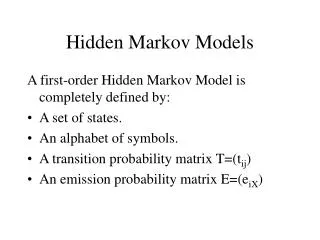
4. Hidden Markov Models • Components: • Observed variables • Emitted symbols • Hidden variables • Relationships between them • Represented by a graph with transition probabilities • Goal: Find the most likely explanation for the observed variables

5. The occasionally dishonest casino • A casino uses a fair die most of the time, but occasionally switches to a loaded one • Fair die: Prob(1) = Prob(2) = . . . = Prob(6) = 1/6 • Loaded die: Prob(1) = Prob(2) = . . . = Prob(5) = 1/10, Prob(6) = ½ • These are the emission probabilities • Transition probabilities • Prob(Fair  Loaded) = 0.01 • Prob(Loaded Fair) = 0.2 • Transitions between states obey a Markov process

6. An HMM for the occasionally dishonest casino

8. The occasionally dishonest casino • Known: • The structure of the model • The transition probabilities • Hidden: What the casino did • FFFFFLLLLLLLFFFF... • Observable: The series of die tosses • 3415256664666153... • What we must infer: • When was a fair die used? • When was a loaded one used? • The answer is a sequenceFFFFFFFLLLLLLFFF...

9. Making the inference • Model assigns a probability to each explanation of the observation: P(326|FFL) = P(3|F)·P(FF)·P(2|F)·P(FL)·P(6|L) = 1/6 · 0.99 · 1/6 · 0.01 · ½ • Maximum Likelihood: Determine which explanation is most likely • Find the path most likely to have produced the observed sequence • Total probability: Determine probability that observed sequence was produced by the HMM • Consider all paths that could have produced the observed sequence

10. Notation • xisthe sequence of symbols emitted by model • xiis the symbol emitted at time i • A path, , is a sequence of states • The i-th state in  is i • akr is the probability of making a transition from state k to state r: • ek(b) is the probability that symbol b is emitted when in state k

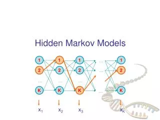
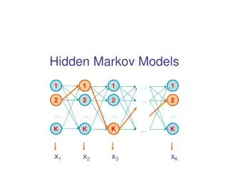
11. 0 0 1 1 1 1 … 2 2 2 2 … … … … … K K K K … A “parse” of a sequence 1 2 2 K x1 x2 x3 xL

12. The occasionally dishonest casino

13. The most probable path The most likely path * satisfies To find *, consider all possible ways the last symbol of x could have been emitted Let Then

14. The Viterbi Algorithm • Initialization (i = 0) • Recursion (i = 1, . . . , L): For each state k • Termination: To find *, use trace-back, as in dynamic programming

15. Viterbi: Example x 2 6  6 0 0 B 1 0 (1/6)max{(1/12)0.99, (1/4)0.2} = 0.01375 (1/6)max{0.013750.99, 0.020.2} = 0.00226875 (1/6)(1/2) = 1/12 0 F  (1/2)max{0.013750.01, 0.020.8} = 0.08 (1/10)max{(1/12)0.01, (1/4)0.8} = 0.02 (1/2)(1/2) = 1/4 0 L

16. Viterbi gets it right more often than not

17. An HMM for CpG islands Emission probabilities are 0 or 1. E.g. eG-(G) = 1, eG-(T) = 0 See Durbin et al., Biological Sequence Analysis,. Cambridge 1998

18. Total probabilty Many different paths can result in observation x. The probability that our model will emit x is Total Probability If HMM models a family of objects, we want total probability to peak at members of the family. (Training)

19. å f ( i ) e ( x ) f ( i 1 ) a = - r i k k rk r Total probability Pr(x) can be computed in the same way as probability of most likely path. Let Then and

20. The Forward Algorithm • Initialization (i = 0) • Recursion (i = 1, . . . , L): For each state k • Termination:

21. The Backward Algorithm • Initialization (i = L) • Recursion (i = L-1, . . . , 1): For each state k • Termination:

22. Posterior Decoding • How likely is it that my observation comes from a certain state? • Like the Forward matrix, one can compute a Backward matrix • Multiply Forward and Backward entries • P(x) is the total probability computed by, e.g., forward algorithm

23. Posterior Decoding With prob 0.05 for switching to the loaded die: With prob 0.01 for switching to the loaded die:

24. Estimating the probabilities (“training”) • Baum-Welch algorithm • Start with initial guess at transition probabilities • Refine guess to improve the total probability of the training data in each step • May get stuck at local optimum • Special case of expectation-maximization (EM) algorithm

25. Baum-Welch algorithm Prob. st used at the position i (for one seq x) Estimated number of transitions st: Estimated number of emissions x from s: New parameter:

26. Profile HMMs • Model a family of sequences • Derived from a multiple alignment of the family • Transition and emission probabilities are position-specific • Set parameters of model so that total probability peaks at members of family • Sequences can be tested for membership in family using Viterbi algorithm to match against profile

27. Profile HMMs

28. Profile HMMs: Example Note: These sequences could lead to other paths. Source: http://www.csit.fsu.edu/~swofford/bioinformatics_spring05/

29. Pfam • “A comprehensive collection of protein domains and families, with a range of well-established uses including genome annotation.” • Each family is represented by two multiple sequence alignments and two profile-Hidden Markov Models (profile-HMMs). • A. Bateman et al. Nucleic Acids Research (2004) Database Issue 32:D138-D141

30. Lab 5 I1 I2 I3 I4 M1 M2 M3 D1 D2 D3

31. Some recurrences I1 I2 I3 I4 M1 M2 M3 D1 D2 D3

32. More recurrences I1 I2 I3 I4 M1 M2 M3 D1 D2 D3