Download
1 / 42
420 likes | 673 Views
Model generalization. Test error Bias, variance and complexity In-sample error Cross-validation Bootstrap “Bet on sparsity ”. Model. Training data. Testing data. Model. Testing error rate. Training error rate.

E N D
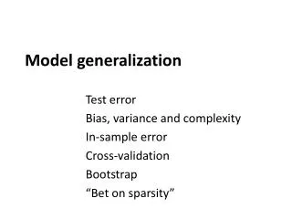
Model generalization Test error Bias, variance and complexity In-sample error Cross-validation Bootstrap “Bet on sparsity”
Model Training data Testing data Model Testing error rate Training error rate Good performance on testing data, which is independent from the training data, is most important for a model. It serves as the basis in model selection.
Test error To evaluate prediction accuracy, loss functions are needed. Continuous Y: In classification, categorical G (class label): Where , Except in rare cases (e.g. 1 nearest neighbor), the trained classifier always gives a probabilistic outcome.
Test error The log-likelihood can be used as a loss-function for general response densities, such as the Poisson, gamma, exponential, log-normal and others. If Prθ(X)(Y) is the density of Y , indexed by a parameter θ(X) that depends on the predictor X, then The 2 makes the log-likelihood loss for the Gaussian distribution match squared error loss.
Test error Test error: The expected loss over an INDEPENDENT test set. The expectation is taken with regard to everything that’s random - both the training set and the test set. In practice it is more feasible to estimate the testing error given a training set: Training error is the average Loss over just the training set:
Test error Test error for categorical outcome: Training error:
Goals in model building Model selection: Estimating the performance of different models; choose the best one (2) Model assessment: Estimate the prediction error of the chosen model on new data.
Goals in model building Ideally, we’d like to have enough data to be divided into three sets: Training set: to fit the models Validation set: to estimate prediction error of models, for the purpose of model selection Test set: to assess the generalization error of the final model A typical split:
Goals in model building What’s the difference between the validation set and the test set? The validation set is used repeatedly on all models. The model selection can chase the randomness in this set. Our selection of the model is based on this set. In a sense, there is over-fitting in terms of this set, and the error rate is under-estimated. The test set should be protected and used only once to obtain an unbiased error rate.
Goals in model building In reality, there’s not enough data. How do people deal with the issue? Eliminate validation set. Draw validation set from training set. Try to achieve generalization error and model selection. (AIC, BIC, cross-validation ……) Sometimes, even omit the test set and final estimation of prediction error; publish the result and leave testing to later studies.
Bias-variance trade-off In the continuous outcome case, assume The expected prediction error in regression is:
Bias-variance trade-off K-nearest neighbor classifier: The higher the k, the lower the model complexity (estimation becomes more global, space partitioned into larger patches) Increase k, the variance term decreases, and the bias term increases. (Here x’s are assumed to be fixed; randomness only in y)
Bias-variance trade-off For linear model with p coefficients, Although h(x0) is dependent on x0, its average over sample values is p/N Model complexity is directly associated with p.
Bias-variance trade-off An example. 50 observations, 20 predictors, uniformly distributed in the hypercube [0, 1]20 Y is 0 if X1 ≤ 1/2 and 1 if X1 > 1/2, and apply k-nearest neighbors. Red: prediction error Green: squared bias Blue: variance
Bias-variance trade-off An example. 50 observations, 20 predictors, uniformly distributed in the hypercube [0, 1]20 Red: prediction error Green: squared bias Blue: variance
In-sample error With limited data, we need to approach testing error (hidden) as much as we can, and/or perform model selection. Two general approaches: Analytical AIC, BIC, Cp, …. (2) Resampling-based Cross-validation, bootstrap, jackknife, ……
In-sample error Training error: This is an under-estimate of the true error Because the same data is used to fit the model and assess the error. Err is extra-sample error, because test data points can come from outside the training set.
In-sample error We will only know Err when we know the population. However, we know only the training sample which is drawn from the population, but not the population itself. In-sample error: obtained when new responses are observed at the same x’s as the training set
In-sample error y Population Sample New sample at same x’s x Define the optimism as For squared error, 0-1, and other loss function, it can be shown generally that
In-sample error • The amount by which Err underestimates the true error depends on how strongly yi affects its own prediction. • Generally, Errinis a better estimate of the test error than the training error, because the in-sample is a better approximation to the population. • So the goal is to estimate the optimism and add it to the training error. (Cp, AIC, BIC work this way for models linear in their parameters.)
In-sample error Cp statistic: AIC: BIC:
In-sample error BIC tends to choose overly simple models when sample size is small; it chooses the correct model when sample size approaches infinity. AIC tends to choose overly complex models when sample size is large.
Cross-validation The goal is to directly estimate the extra-sample error (error on an independent test set) K-fold cross-validation: Split data into K roughly equal-sized parts For each of the K parts, fit the model with the other K-1 parts, and calculate the prediction error on the part that is left out.
Cross-validation The CV estimate of the prediction error is from the combination of the K estimates α is the tuning parameter (different models, model parameters) Find that minimizes CV(α) Finally, fit all data on the model
Cross-validation CV could substantially over-estimate prediction error, depending on the learning curve.
Cross-validation Leave-one-out cross-validation (K=N) is approximately unbiased, yet it has high variance. K=5 or 10, CV has low variance but more bias. If the learning curve has large slope at the training set size, a 5-fold or 10-fold CV can overestimate the prediction error substantially.
Cross-validation In multi-stage modeling. Example: 5000 genes, 50 normal/50 disease subjects ? Select 100 genes that best correlate with disease status CV error rate: 3%. 5-fold CV. The 100 genes don’t change; model parameters are tuned Build a multivariate predictor using the 100 genes.
Cross-validation 5-fold CV Split the data. For each fold – Select 100 genes using 4/5 of the samples. Build a classification model using the 4/5 samples. Predict the other 1/5 samples.
Bootstrap Resample the training set to generate B bootstrap samples. Fit the model on each of the B samples. Examine prediction accuracy for each observation from those models not built from the observation. For example the leave-one-out bootstrap estimate of prediction error is
Bootstrap Reminder: in bootstrap, each sample has the probability of 0.632 of being selected into a re-sample. Average number of distinct observations in a bootstrap sample is 0.632N. The (upward) bias will behave like a two-fold cross-validation.
Bootstrap The 0.632 estimator can alleviate the bias Intuitively it pulls the upward biased leave-one-out error rate towards the downward biased training set error rate.
“Bet on sparsity” principle L1 penalty yields sparse models. L2 penalty yields dense models, and is computationally easy. When underlying model is sparse, L1 penalty does well. When underlying model is dense, and the training data size is not extremely large, neither does well because of the curse of dimensionality. “Use a procedure that does well in sparse problems, since no procedure does well in dense problems”
“Bet on sparsity” principle Example, 300 predictors, 50 observations, Dense scenario: all 300 betas are non-zero Sparse scenario: only 10 betas are non-zero 30 betas are non-zero
“Bet on sparsity” principle Data generated from dense model – neither do well.
“Bet on sparsity” principle Date generated from sparse model – Lasso does well.
“Bet on sparsity” principle Date generated from relatively sparse model – Lasso does better than ridge.