16.2: Line Integrals 16.3: The Fundamental Theorem for Line Integrals

1. 16.2:Line Integrals • 16.3:The Fundamental Theorem for Line Integrals • 16.5:Curl and Divergence

2. 16.2 • Line Integrals

3. Line Integrals • A Line Integral is similar to a single integral except that instead of integrating over an interval [a, b], we integrate over a curve C. • Just as for an ordinary single integral, we can interpret the line integral of a positive function as an area. • In fact, if f (x, y)  0, Cf (x, y) ds represents the area of one side of the “fence” or “curtain”, whose base is C and whose height above the point (x, y) is f (x, y):

4. Line Integrals or “Curve Integrals” • Line integrals were invented in the early 19th century to solve problems involving fluid flow, forces, electricity, and magnetism. • We start with a plane curve C given by: • the parametric equations: x = x(t) y = y(t) a t b • or the vector equation: r(t) = x(t) i+ y(t) j, • and we assume that C is a smooth curve. [Meaning r is continuous and r(t)0.]

5. Example: • Consider the function f = x+y and the parabola y=x2 in the x-y plane, for 0≤ x ≤2. • Imagine that we extend the parabola up to the surface f, to form a curved wall or curtain: • The base of each rectangle is the arc length along the curve: ds • The height is the value of fabove the arc length. • If we add up the areas of these rectangles as we move along the curve C, we get the area: Parabola is the curve C

6. Example (cont.’) • Next: Rewrite the function f(x,y) after parametrizing x and y: • For example in this case, we can choose: x(t) =t and y(t) = t2 • So r = <t, t2> and f = t +t2 • using the fact that (recall from chapter 13! ) • ds = | r’ | dt • then ds = • And the integral becomes:

7. Line Integrals in 2D: • The Line integral of f along C is given by: • NOTE: • The value found for the line integral will not depend on the parametrization of the curve, provided that the curve is traversed exactly once as t increases from a to b.

8. Practice 1: • Evaluate C (2 + x2y) ds, where C is the upper half of the unit circle • x2 + y2 = 1. • Solution: • In order to use Formula 3, we first need parametric equations to represent C. • Recall that the unit circle can be parametrized by means of the equations • x = cos t y = sin t • and the upper half of the circle is described by the parameter interval 0t .

9. Practice 1 – Solution • cont’d • Therefore Formula 3 gives

10. Application: • If f(x, y) = 2 + x2yrepresents the density of a semicircular wire, then the integral in Example 1 would represent the mass of the wire! • The center of mass of the wire with density function  is located at the point , where

11. Line Integrals in 3D Space: • We now suppose that C is a smooth space curve given by the parametric equations: • x = x(t) y = y(t) z = z(t) a t b • or by a vector equation: • r(t) = x(t) i + y(t) j + z(t) k. • If f is a function of three variables that is continuous on some region containing C, then we define the line integral of f along C (with respect to arc length) in a manner similar to that for plane curves:

12. Line Integrals • Notice that in both 2D or 3D the compact form of writing a line integral is: • For the special case f (x, y, z) = 1, we get: • Which is simply the length of the curve C!

13. Example: • Evaluate C y sin zds, where C is the circular helix given by the equations: x = cos t, y = sin t, z = t, 0 t 2.

14. Example – Solution • Formula 9 gives:

15. Line Integrals of Vector Fields • Suppose that F = P i + Q j + R k is a continuous force field. • The work done by this force in moving a particle along a smooth curve C is: • Equation 12 says that work is the line integral with respect to arc length of the tangential component of the force. • This integral is often abbreviated as CF drand occurs in other areas of physics as well.

16. Example • Find the work done by the force field F(x, y) = x2 i – xyj • in moving a particle along the quarter-circle • r(t) = cos ti + sin tj, 0 t/2. • Solution: • Since x = cos t and y = sin t, we have • F(r(t)) = cos2t i –cos t sin t j • and r(t) = –sin t i + cos t j

17. Example – Solution cont’d • Therefore the work done is

18. 16.3 • The Fundamental Theorem for Line Integrals

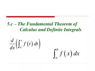
19. The Fundamental Theorem for Line Integrals • Recall that Part 2 of the Fundamental Theorem of Calculus can be written as: • where F is continuous on [a, b]. • This is also called: the Net Change Theorem.

20. The Fundamental Theorem for Line Integrals • If we think of the gradient vector f of a function f of two or three variables as a sort of derivative of f, then the following theorem can be regarded as a version of the Fundamental Theorem for line integrals:

21. Example 1 • F is called a “conservative” vector field if it can be written as: F =f

22. Example 1 – Solution • cont’d • Therefore, by Theorem 2, the work done is • W = CF dr • = Cfdr • = f (2, 2, 0) – f (3, 4, 12)

23. Curl and Divergence • 16.5

24. Curl • If F = P i + Q j + R k is a vector field on and the partial • derivatives of P, Q, and R all exist, then the curl of F is the • vector field defined by: • Let’s rewrite Equation 1 using operator notation. We introduce the vector differential operator  (“del”) as:

25. Curl • It has meaning when it operates on a scalar function to produce the gradient of f : • If we think of  as a vector with components ∂/∂x, ∂/∂y, and ∂/∂z, we can also consider the formal cross product of  with the vector field F as follows:

26. Curl • So the easiest way to remember Definition 1 is by means of the symbolic expression

27. Example 1 • If F(x, y, z) = xz i + xyz j – y2k, find curl F. • Solution: • Using Equation 2, we have

28. Example 1 – Solution • cont’d

29. Property of Curl: • F is called a “conservative” vector field if it can be written as: F =f • The following theorems says that the curl of a gradient vector field is 0.

30. Why the name: Curl • When F represents the velocity field in fluid flow. Particles near (x, y, z) in the fluid tend to rotate about the axis that points in the direction of curl F(x, y, z), and the length of this curl vector is a measure of how quickly the particles move around the axis. • If curl F = 0 at a point P, then the fluid is free from rotations at P and F is called irrotational at P. • In other words, there is no whirlpool or eddy at P.

31. Divergence • If F = P i + Q j + R k is a vector field on and ∂P/∂x, ∂Q/∂y, and ∂R/∂z exist, then the divergence of F is the function of three variables defined by • NOTE: that curl F is a vector but div F is a scalar!

32. Divergence • In terms of the gradient operator  = (∂/∂x)i + (∂/∂y) j + (∂/∂z) k, the divergence of F can be written symbolically as the dot product of  and F:

33. Example 2 • If F(x, y, z)=xzi + xyzj +y2k, find div F. • Solution: • By the definition of divergence (Equation 9 or 10) we have • div F = F • = z + xz

34. Property of Divergence: • If F is a vector field on , then curl F is also a vector field • on . As such, we can compute its divergence. • The next theorem shows that the result is 0.

35. Why the name “Divergence” • If F(x, y, z) is the velocity of a fluid (or gas), then div F(x, y, z) represents the net rate of change (with respect to time) of the mass of fluid (or gas) flowing from the point (x, y, z) per unit volume. • So div F(x, y, z) measures the tendency of the fluid to diverge from the point (x, y, z). • If div F = 0, then F is said to be incompressible.

36. Div of Gradient: Laplace operator • If f is a function of three variables, we have • and this expression occurs so often that we abbreviate it as 2f. The operator: 2 =  • 2is called the Laplace operator because of its relation to Laplace’s equation:

37. Laplace operator: • We can also apply the Laplace operator 2 to a vector field • F = P i + Q j + R k • in terms of its components: • 2F = 2P i + 2Q j + 2R k

38. Summary of operators:

39. Maxwell’s equations: • Definition of terms: