Techniques for Cash Flow Analysis
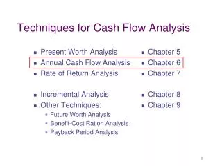
Techniques for Cash Flow Analysis. Present Worth Analysis Annual Cash Flow Analysis Rate of Return Analysis Incremental Analysis Other Techniques: Future Worth Analysis Benefit-Cost Ration Analysis Payback Period Analysis. Chapter 5 Chapter 6 Chapter 7 Chapter 8 Chapter 9.

Techniques for Cash Flow Analysis
E N D
Presentation Transcript
Techniques for Cash Flow Analysis • Present Worth Analysis • Annual Cash Flow Analysis • Rate of Return Analysis • Incremental Analysis • Other Techniques: • Future Worth Analysis • Benefit-Cost Ration Analysis • Payback Period Analysis • Chapter 5 • Chapter 6 • Chapter 7 • Chapter 8 • Chapter 9
Techniques for Cash Flow Analysis SA A A A A Present Worth Analysis: PVA(0)=-RA+A(P/A,i,n)+SA(P/F,i,n) PVB(0)=-RB+B(P/A,i,n)+SB(P/F,i,n) If PVA(0)>PVB(0) => choose A, otherwise => choose B. Annual Cash Flow Analysis: EUACA=RA(A/P,i,n) EUABA=A+SA(A/F,i,n) (EUAB-EUAC)A=A+SA(A/F,i,n)- RA(A/P,i,n) (EUAB-EUAC)B=B+SB(A/F,i,n)- RB(A/P,i,n) If (EUAB-EUAC)A>(EUAB-EUAC)B => choose A, otherwise => choose B. 0 1 2 3 … n RA B B B B SB 0 1 2 3 … n RB (EUAB-EUAC)A (EUAB-EUAC)A (EUAB-EUAC)B (EUAB-EUAC)B (EUAB-EUAC)A (EUAB-EUAC)A (EUAB-EUAC)A (EUAB-EUAC)B (EUAB-EUAC)B (EUAB-EUAC)B 0 1 2 3 … n 0 1 2 3 … n
Example 6-2 A student bought $1000 worth of home furniture. It is expected to last 10 year. The student believes that the furniture can be sold at the end of 10 years for $200. what will the equivalent uniform annual cost be if interest is 7%? S = 200 4 5 6 7 8 9 10 0 1 2 3 P = 1000 Solution 1 EUAC = P(A/P, i , n) – S(A/F, i, n) = 1000(A/P, 7%, 10) – 200(A/F, 7%, 10) = 1000(0.1424) – 200(0.0724) = 142.40 – 14.48 = $127.92
… Example 6-2 Solution 2 Recall that (A/P, i, n) = (A/F, i, n) + i and EUAC = P(A/P, i , n) – S(A/F, i, n) then: EUAC = P(A/F, i, n) + Pi – S(A/F, i, n) = (P – S)(A/F, i, n) + Pi = (1000 – 200)(A/F, 7%, 10) + 1000(0.07) = 800(0.0724) + 1000(0.07) = $127.92 Solution 3 Recall that (A/P, i, n) = (A/F, i, n) + i and EUAC = P(A/P, i , n) – S(A/F, i, n) then: EUAC = P(A/P, i, n) – S(A/P, i, n) + Si = (P – S)(A/P, i, n) + Si = (1000 – 200)(A/P, 7%, 10) + 200(0.07) = 800(0.1424) + 200(0.07) = $127.92
Conclusions from example 6-2 When there is an initial disbursement P followed by a salvage value S, the annual cost may be computed any of the three different ways introduced in example 6-2: EUAC = P(A/P, i , n) – S(A/F, i, n) EUAC = (P – S)(A/F, i, n) + Pi EUAC = (P – S)(A/P, i, n) + Si S 4 0 1 2 3 … n P
Analysis Period? 1) Analysis period equal to alternative lives (no problem) 2) Analysis period a common multiple of alternative lives 3) Analysis period for a continuing requirement 4) Infinite analysis period
1) Analysis Period Equals to Alternative Lives When the analysis period for an economy study is the same as the useful life for each alternative, we have an ideal situation. There are no difficulties.
2) Analysis Period = Common Multiple of Alternative Lives Example 6-7 Two pumps are being considered for purchase. If interest is 7%, which pump should be bought. Assume that Pump B will be replaced after its useful life by the same one EUACA = $7,000 (A/P, 7%, 12) - $1,500 (A/F, 7%, 12) EUACB = $5,000 (A/P, 7%, 6) - $1,000 (A/F, 7%, 6) EUACA = $797 EUACB = $909 Under the circumstances of identical replacement, it is appropriate to compare the annual cash flows computed for alternatives based on their own different service lives (12 years, 6 years). $1,500 0 1 2 3 4 5 6 7 8 9 10 11 12 $7,000 $1,000 $1,000 0 1 2 3 4 5 6 7 8 9 10 11 12 $5,000 $5,000 replace B Choose Pump A
3) Analysis Period for a Continuing Requirement Many times the economic analysis is to determine how to provide for a more or less continuing requirement. There is no distinct analysis period. The analysis period is assumed to be long but undefined. In case when alternatives were compared based on PW analysis, the least common multiple of alternative lives was found, and present worth for that time is calculated. In case alternatives are compared based on annual cash flow analysis, it is appropriate to compare the annual cash flows computed for alternatives based on their own different service lives. Example 6-8 EUACA = (7000 – 1500)(A/P, 7%, 12) + 1500(0.07) = $797 EUACB = (5000 – 1000)(A/P, 7%, 9) + 1000(0.07) = $684 For minimum EUAC, select pump B.
4) Infinite Analysis Period Motivating Example Consider the following three mutually exclusive alternatives: Assuming that Alternatives B and C are replaced with identical replacements at the end of their useful lives, and an 8% interest rate, which alternative should be selected? Case 1. We have alternatives with limited (finite) lives in an infinite analysis period situation: If we assume identical replacement (all replacements have identical cost, performance, etc.) then we will obtain the same EUAC for each replacement of the limited-life alternative. The EUAC for the infinite analysis period is therefore equal to the EUAC for the limited life situation. With identical replacement: EUACfor infinite analysis period = EUAC for limited life n EUACB= $150(A/P,8%,20) - $17.62 EUACC= $200(A/P,8%,5) - $55.48
…Infinite Analysis Period Case 2. Another case occurs when we have an alternative with an infinite life in a problem with an infinite analysis period, which is the case in alt. A. In this case, For Alternative A: EUACfor infinite analysis period = P (A/P,i,) + any other annual (costs-benefits) (A/P,i,) = i EUACA= $100(A/P,8%,) - $10.00 = $100 *0.08 - $10.00 = $-2.00 EUACB= $150(A/P,8%,20) - $17.62 = $150*0.1019- $17.62 =$-2.34 EUACC= $200(A/P,8%,5) - $55.48 = $200*2.505 - $55.48 =$-5.38 Example 6-9 in your text explains a similar situation
Example 6-9 Tunnel EUAC = P(A/P, i , ∞) = Pi = $5.5 (0.06) = $330,000 Pipeline EUAC = $5 million(A/P, 6%, 50) = 5M (0.0634) = $317,000 To minimize the EUAC, select the pipeline
Some other analysis period The analysis period may be something other than one of the four cases we describe. It may be equal to the life of the shorter-life alternative, the longer-life alternative, or something entirely different. This is the most general case for annual cash flow analysis. i.e. when the analysis period and the lifetimes of the alternatives of interest are all different. In this case, terminal values at the end of the analysis period become very important. (Example 6-10)
…Some other analysis period (See example 6-10) Alternative 1 = initial cost = salvage value = replacement cost = terminal value at the end of 10th year Alternative 2 = initial cost = terminal value at the end of 10th year Present worth of costs with 10-yr. analysis period: EUAC1 = [C1 + (R1 – S1)(P/F,i%,7) – T1 (P/F,i%,10)] (A/P, i, 10) EUAC2 = [C2 – T2 (P/F,i%, 10)] (A/P, i, 10) 7 years 3 years 3 years 1 year