Download

1 / 47
470 likes | 809 Views
t scores and confidence intervals using the t distribution. What we will cover today:. t scores as estimates of z scores; t curves as approximations of z curves Estimated standard errors CIs using the t distribution Testing the no effect (null) hypothesis).

E N D
What we will cover today: t scores as estimates of z scores; t curves as approximations of z curves Estimated standard errors CIs using the t distribution Testing the no effect (null) hypothesis)
Simply substitute X for mu and s for sigma. That is, substitute estimates for parameters. t scores indicate the distance and direction of a score from the sample mean. • t scores are computed like Z scores.
More t scores • As long as the raw scores are obtained from a random sample, then t scores are least squares, unbiased, consistent estimators of what the Z scores would be if we had all the scores in the population. Any score can be translated to a t scores as long as you can estimate mu and sigma with X-bar and s.
score – estimated mean t = Estimated standard deviation 6’ - 5’8” t = 3” 72 - 68 4 1.33 = = = 3 3 Calculating t scores What is the t score for someone 6’ tall, if the sample mean is 5’8” and the estimated standard deviation is 3 inches (s=3”)?
Body and tails of the curve • The body of a curve is the area enclosed in a symmetrical interval around the mean. • The tails of a curve are the two regions of the curve outside of the body. • The critical values of the t curves are the number of estimated standard deviations one must go from the mean to reach the point where 95% or 99% of the curve is enclosed in a symmetrical interval around the mean (in the body) and 5% or 1% is in the two tails combined. • The critical values of the t curve change depending on how many df there are for MSW and s.
We can define a curve by stating its critical values • The Z curve can be defined as one of the family of t curves in which 95% of the curve falls within 1.960 standard deviations from the mean and 99% falls within 2.576 standard deviations from the mean. • We can define t curves in terms of how many estimated standard deviations you must go from the mean before the body of the curve contains 95% and 99% of the curve and the combined upper and lower tails contain 5% and 1% respectively.
t curves • t curves are used instead of the Z curve when you are using samples to estimate sigma2 with MSW. • Since we are estimating sigma instead of knowing it, t curves are based on less information than the Z curve. • Therefore, t curves partake somewhat of the rectangular (“I know nothing”) distribution and tend to be flatter than the Z curve. • The more degrees of freedom for MSW, the better our estimate of sigma2. • The better our estimate, the more t curves resemble Z curves.
5 df 1 df Standard deviations 3 2 1 0 1 2 3 To get 95% of the population in the body of the curve when there are 5 df of freedom, you go out over 3 standard deviations. To get 95% of the population in the body of the curve when there is 1 df of freedom, you go out over 12 standard deviations. t curves and degrees of freedomZ curve F r e q u e n c y score
Critical values of the t curves • The following table defines t curves with 1 through 10,000 degrees of freedom • Each curve is defined by how many estimated standard deviations you must go from the mean to define a symmetrical interval that contains a proportions of .9500 and .9900 of the curve, leaving proportions of .0500 and .0100 in the two tails of the curve (combined). • Values for .9500/.0500 are shown in plain print. Values for .9900/.0900 and the degrees of freedom for each curve are shown in bold print.
df 1 2 3 4 5 6 7 8 .05 12.706 4.303 3.182 2.776 2.571 2.447 2.365 2.306 .0163.657 9.925 5.841 4.604 4.032 3.707 3.499 3.355 df 9 10 11 12 13 14 15 16 .05 2.262 2.228 2.201 2.179 2.160 2.145 2.131 2.120 .013.250 3.169 3.106 3.055 3.012 2.997 2.947 2.921 df 17 18 19 20 21 22 23 24 .05 2.110 2.101 2.093 2.086 2.080 2.074 2.069 2.064 .012.898 2.878 2.861 2.845 2.831 2.819 2.807 2.797 df 25 26 27 28 29 30 40 60 .05 2.060 2.056 2.052 2.048 2.045 2.042 2.021 2.000 .012.787 2.779 2.771 2.763 2.756 2.750 2.704 2.660 df 100 200 500 1000 2000 10000 .05 1.984 1.972 1.965 1.962 1.961 1.960 .012.626 2.601 2.586 2.581 2.578 2.576
Using the t table You can answer things like: • If we have 13 degrees of freedom then how far do we have to go above the mean in order to have only 5% of the curve left in the tails? (Answer: Out to a t score of 2.160) • How many estimated standard deviations do we have to go out in order to leave 1% of the scores in the tails with 3 degrees of freedom? (Answer: 5.841) • With 10 degrees of freedom and a critical value of .05, is a t score of -2.222 inside the body or the tail of the t curve? How about with 11 df. (Answer: With 10 df, inside the body. With 11 df outside the body in the tail.) • What are the critical values of a t curve with 20 df? (Answer: 2.086 at .95/.05 and 2.845 at .99/.01.)
df 1 2 3 4 5 6 7 8 .05 12.706 4.303 3.182 2.776 2.571 2.447 2.365 2.306 .0163.657 9.925 5.841 4.604 4.032 3.707 3.499 3.355 df 9 10 11 12 13 14 15 16 .05 2.262 2.228 2.201 2.179 2.160 2.145 2.131 2.120 .013.250 3.169 3.106 3.055 3.012 2.997 2.947 2.921 df 17 18 19 20 21 22 23 24 .05 2.110 2.101 2.093 2.086 2.080 2.074 2.069 2.064 .012.898 2.878 2.861 2.845 2.831 2.819 2.807 2.797 df 25 26 27 28 29 30 40 60 .05 2.060 2.056 2.052 2.048 2.045 2.042 2.021 2.000 .012.787 2.779 2.771 2.763 2.756 2.750 2.704 2.660 df 100 200 500 1000 2000 10000 .05 1.984 1.972 1.965 1.962 1.961 1.960 .012.626 2.601 2.586 2.581 2.578 2.576
A slightly harder problem type: with a single sample (n=22), you have 21 df for MSW and therefore for the t curve. Say your t score = +2.080, what percentile would you be at? (Hint: the answer is not the 95th percentile.)
df 1 2 3 4 5 6 7 8 .05 12.706 4.303 3.182 2.776 2.571 2.447 2.365 2.306 .0163.657 9.925 5.841 4.604 4.032 3.707 3.499 3.355 df 9 10 11 12 13 14 15 16 .05 2.262 2.228 2.201 2.179 2.160 2.145 2.131 2.120 .013.250 3.169 3.106 3.055 3.012 2.997 2.947 2.921 df 17 18 19 20 21 22 23 24 .05 2.110 2.101 2.093 2.086 2.080 2.074 2.069 2.064 .012.898 2.878 2.861 2.845 2.831 2.819 2.807 2.797 df 25 26 27 28 29 30 40 60 .05 2.060 2.056 2.052 2.048 2.045 2.042 2.021 2.000 .012.787 2.779 2.771 2.763 2.756 2.750 2.704 2.660 df 100 200 500 1000 2000 10000 .05 1.984 1.972 1.965 1.962 1.961 1.960 .012.626 2.601 2.586 2.581 2.578 2.576
A slightly harder problem: with a single sample (n=22), you have 21 df for MSW and therefore for the t curve. Say your t score = +2.080, what percentile would you be at? 98th percentile (50 + 47.5 = 97.5 = 98th percentile)
Estimated distance of sample means from mu: estimated standard errors of the mean • We can compute the standard error of the mean when we know sigma. • We just have to divide sigma by the square root of n, the size of the sample • Similarly, we can estimate the standard error of the mean, estimate the average unsquared distance of sample means from mu. • We just have to divide s by the square root of n, the size of the sample in which we are interested
Note that the estimated standard error is determined by only two factors: the estimated average unsquared distance of scores from mu (s) and the size of the sample (n).
Look at the effects of increased variation and increased sample size in the next slide. • In the first set of computations on the next slide, n stays constant while s and the estimated standard error increase. • In the second set of computations on the next slide, s stays constant while n increases and the estimated standard error decreases.
s n • A 2.83 8 1.00 = 2.83/2.83 • B 12.00 8 4.24 = 12.00/2.83 • C 20.00 8 7.07 = 20.00/2.83 • D 2.83 1 2.83 = 2.83/1.00 • E 2.83 2 2.00 = 2.83/1.41 • F 2.83 8 1.00 = 2.83/2.83 • G 2.83 40 0.45 = 2.83/6.32
There are two reasons to create confidence intervals with the t distribution • 1. To test a theory about what mu is. (We call the theoretical population means muT). • THAT’S THE IMPORTANT REASON AND WE WILL LEARN ABOUT IT FIRST • 2. The other reason is to define an interval in which we are confident mu would fall if we knew it.
Confidence intervals around muT and testing the null hypothesis
Confidence intervals and hypothetical means • We frequently have a theory about what the mean of a distribution should be. • To be scientific, that theory about mu must be able to be proved wrong (falsified). • One way to test a theory about a mean is to state a range where sample means should fall if the theory is correct. • We usually state that range as a 95% confidence interval.
To test our theory, we take a random sample from the appropriate population and see if the sample mean falls where the theory says it should, inside the confidence interval. • If the sample mean falls outside the 95% confidence interval established by the theory, the evidence suggests that our theoretical population mean and the theory that led to its prediction is wrong. • When that happens our theory has been falsified. We must discard it and look for an alternative explanation of our data.
For example: • For example, let’s say that we had a new antidepressant drug we wanted to peddle. Before we can do that we must show that the drug is safe. • Drugs like ours can cause problems with body temperature. People can get chills or fever. • We want to show that body temperature is not effected by our new drug.
Testing a theory • “Everyone knows” that normal body temperature for healthy adults is 98.6oF. • Therefore, it would be nice if we could show that after taking our drug, healthy adults still had an average body temperature of 98.6oF. • So we might test a sample of 16 healthy adults, first giving them a standard dose of our drug and, when enough time had passed, taking their temperature to see whether it was 98.6oF on the average.
Testing a theory - 2 • Of course, even if we are right and our drug has no effect on body temperature, we wouldn’t expect a sample mean to be precisely 98.600000… • We would expect some sampling fluctuation around a population mean of 98.6oF.
Testing a theory - 3 • So, if our drug does not cause change in body temperature, the sample mean should be close to 98.6. It should, in fact, be within the 95% confidence interval around a theoretical mean of 98.6. • SO WE MUST CONSTRUCT A 95% CONFIDENCE INTERVAL AROUND 98.6o AND SEE WHETHER OUR SAMPLE MEAN FALLS INSIDE OR OUTSIDE THE CI.
To create a confidence interval around muT, we must estimate sigma from a sample. • We randomly select a group of 16 healthy individuals from the population. • We administer a standard clinical dose of our new drug for 3 days. • We carefully measure body temperature. • RESULTS: We find that the average body temperature in our sample is 99.5oF with an estimated standard deviation of 1.40o (s=1.40). • IS 99.5oF. IN THE 95% CI AROUND MUT???
Knowing s and n we can easily compute the estimated standard error of the mean. • Let’s say that s=1.40o and n = 16: • = 1.40/4.00 = 0.35 • Using this estimated standard error we can construct a 95% confidence interval for the body temperature of a sample of 16 healthy adults.
We learned how to create confidence intervals with the Z distribution in Chapter 4. 95% of sample means will fall in a symmetrical interval around mu that goes from 1.960 standard errors below mu to 1.960 standard errors above mu • A way to write that fact in statistical language is: CI.95: mu + ZCRIT* sigmaX-bar or CI.95: mu - ZCRIT* sigmaX-bar < X-bar < mu + ZCRIT* sigmaX-bar For a 95% CI, ZCRIT = 1.960
But when we must estimate sigma with s, we must use the t distribution to define critical intervals around mu or muT. Here is how we would write the formulae substituting t for Z and s for sigma CI95: muT+ tCRIT* sX-bar or CI.95: muT - tCRIT* sX-bar < X-bar < muT + tCRIT* sX-bar
Notice that the critical value of t that includes 95% of the sample means changes with the number of degrees of freedom for s, our estimate of sigma, and must be taken from the t table.If n= 16 in a single sample, dfW=n-k=15.
df 1 2 3 4 5 6 7 8 .05 12.706 4.303 3.182 2.776 2.571 2.447 2.365 2.306 .0163.657 9.925 5.841 4.604 4.032 3.707 3.499 3.355 df 9 10 11 12 13 14 15 16 .05 2.262 2.228 2.201 2.179 2.160 2.145 2.131 2.120 .013.250 3.169 3.106 3.055 3.012 2.997 2.947 2.921 df 17 18 19 20 21 22 23 24 .05 2.110 2.101 2.093 2.086 2.080 2.074 2.069 2.064 .012.898 2.878 2.861 2.845 2.831 2.819 2.807 2.797 df 25 26 27 28 29 30 40 60 .05 2.060 2.056 2.052 2.048 2.045 2.042 2.021 2.000 .012.787 2.779 2.771 2.763 2.756 2.750 2.704 2.660 df 100 200 500 1000 2000 10000 .05 1.984 1.972 1.965 1.962 1.961 1.960 .012.626 2.601 2.586 2.581 2.578 2.576
So, muT=98.6, s=1.40, n=16, df = 15, tCRIT=2.131 Here is the confidence interval: CI.95: muT+ tCRIT* sX-bar = = 98.6 + (2.131)*(1.40/ ) = = 98.6 + (2.131)*(1.40/4) = 98.6 + (2.131)(0.35) =98.60+ 0.75 CI.95: 97.85< X-bar < 99.35
CI.95: 97.85< X-bar < 99.35: The confidence interval consistent with the theory that our drug does not casues a change in body temperature goes from 97.85o to 99.35o. Our sample mean was 99.5o F. So, our sample mean falls outside the CI.95 and falsifies the theory that our drug has no effect on body temperature. Our drug may cause a slight fever.
Testing the no-effect (null) hypothesis • Specify what you believe the value of a statistic will be if your idea of the situation is correct. In this case, you specified muT=98.6o F. • Define a 95% Confidence Interval around that value of your test statistic. • See if the test statistic falls inside the CI.95 • If it falls within the CI.95, you retain the no-effect hypothesis • If it falls outside the CI.95, you reject the no effect hypothesis. Further, if you then have to guess what the true value of the test statistic is in the population as a whole, you chose the value that was found in the random sample.
THE FOLLOWING MATERIAL IS LESS IMPORTANT AND WILL ONLY BE GONE OVER IF THERE IS EXTRA TIME. MAKE SURE YOU UNDERSTAND TESTING THE NO EFFECT HYPOTHESIS BEFORE GOING ON.
Since Chapter 1 you have been making least squared, unbiased estimates • You have learned to predict that everyone would score at a specific point. This is called “making point estimates.” • The point estimates have been wrong in a least squared, consistent, unbiased way. • If you want to be right, not wrong, you can’t make point estimates, you must make interval estimates.
Interval estimates of mu • As you know, X-bar is our least squared, unbiased, consistent estimate of mu. • To create an interval estimate of mu, we create a symmetrical interval around X-bar. • We usually create 95% and/or 99% CIs to define that interval.
The generic formula for confidence intervals for mu CI: X-bar + (tCRIT* sX-bar )or CI: X-bar – tCRIT* sX-bar < mu< X-bar+ tCRIT* sX-bar If we use the critical values of t at .95 we will have an interval that includes mu if our sample is one of the 95% that falls within a 95% CI around mu. If we use the critical values of t at .99 we will have an interval that includes mu if our sample is one of the 95% that falls within a 99% CI around mu.
Here is an example • Let’s say (because professors know everything) that I knew that the average height of all male Rutgers Juniors is 70.0 inches (5’10”) • I assign you, the student to take a sample of 16 male Rutgers Juniors and measure their height. • Then you must define an interval in which mu should be found. • You find that X-bar = 69.3” and s = 2.00 inches.
df 1 2 3 4 5 6 7 8 .05 12.706 4.303 3.182 2.776 2.571 2.447 2.365 2.306 .0163.657 9.925 5.841 4.604 4.032 3.707 3.499 3.355 df 9 10 11 12 13 14 15 16 .05 2.262 2.228 2.201 2.179 2.160 2.145 2.131 2.120 .013.250 3.169 3.106 3.055 3.012 2.997 2.947 2.921 df 17 18 19 20 21 22 23 24 .05 2.110 2.101 2.093 2.086 2.080 2.074 2.069 2.064 .012.898 2.878 2.861 2.845 2.831 2.819 2.807 2.797 df 25 26 27 28 29 30 40 60 .05 2.060 2.056 2.052 2.048 2.045 2.042 2.021 2.000 .012.787 2.779 2.771 2.763 2.756 2.750 2.704 2.660 df 100 200 500 1000 2000 10000 .05 1.984 1.972 1.965 1.962 1.961 1.960 .012.626 2.601 2.586 2.581 2.578 2.576
So, X-bar=69.3, s=2.00, n=16,df = 15, tCRIT=2.131. Here is the 95% confidence interval. CI.95: X-bar + tCRIT* sX-bar = = 69.3 + (2.131)*(2.00/ ) = = 69.3 + (2.131)*(2.00/4) = 69.3 + (2.131)(0.50) =69.30+ 1.16 CI.95: 68.14< mu< 70.46 In this example, we knew mu ahead of time (70.0) and the computations were just an exercise. But exercise or not, our interval does include mu.
Here is a 99% CI with the same data X-bar=69.3, s=2.00, n=16, df = 15, tCRIT=2.947 CI.99: X-bar + tCRIT* sX-bar = = 69.3 + (2.947)*(2.00/4) = 69.3 + (2.947)(0.50) =69.30+ 1.47 CI.99: 67.83< mu< 70.77 Of course, since we have to go further out into the tails of the curve to include 99% of the sample means, the interval for the CI99 is wider (less precise) that the interval for the CI.95 .