Download
1 / 11
110 likes | 249 Views
Statistical modelling and latent variables (2). Mixing latent variables and parameters in statistical inference. State spaces.

E N D
Statistical modelling and latent variables (2) Mixing latent variables and parameters in statistical inference
State spaces We typically have a parametric model for the latent variables, representing the true state of a system. Also, the distribution of the observations may depend on parameters as well as latent variables. Observations may often be seen as noisy versions of the actual state of a system. Examples of states could be: • The physical state of a rocket (position, orientation, velocity, fuel-state). • Real water temperature (as opposed to measured temperature). • Occupancy in an area. • Carrying capacity in an area. Use green arrows for one-way parametric dependency (for which you don’t provide a probability distribution in frequentist statistics). L D
Observations, latent variables and parameters - inference Sometimes we are interested in the parameters, sometimes in the state of the latent variables, sometimes both. Impossible to do inference on the latent variables without also dealing with the parameters and vice versa. D L Often, other parameters affect the latent variables than the observations. L L D D
Observations, latent variables and parameters ML estimation A latent variable model will specify the distribution of the latent variables given the parameters and the distribution of the observations given both the parameters and the latent variables. This will give the distribution of data *and* latent variables: f(D,L|)=f(L|)f(D|L,) But in an ML analysis, we want the likelihood, f(D|)! Theory (law of total probability again): L D
Observations, latent variables and parameters ML estimation Likelihood: The integral can often not be obtained analytically. In occupancy, the sum is easy (only two possible states) Kalman filter: For latent variables as linear normal Markov chains with normal observations depending linearly on them, this can be done analytically. Alternative when analytical methods fail: numerical integration, particle filters, Bayesian statistics using MCMC.
Occupancy as a state-space model – the model in words Assume a set areas, i(1,…,A). Each area has a set of nitransects. Each transect has an independent detection probability, p, given the occupancy. Occupancy is a latent variable for each area, i. Assume independency between the occupancy state in different areas. The probability of occupancy is labelled . So, the parameters are =(p,). Pr(i=1|)=. Start with distribution of observations given the latent variable: Pr(xi,j=1 | i=1,)=p. Pr(xi,j=0 | i=1,)=1-p, Pr(xi,j=1 | i=0,)=0. Pr(xi,j=0 | i=0,)=1. So, for 5 transects with outcome 00101, we will get Pr(00101 | i=1,)=(1-p)(1-p)p(1-p)p=p2(1-p)3. Pr(00101 | i=0,)=11010=0
Occupancy as a state-space model – graphic model =occupancy rate p=detection rate given occupancy. p Parameters (): Pr(i=1|)= Pr(i=0|)=1- 1 2 3 A One latent variable per area (area occupancy) ……… The area occupancies are independent. Pr(xi,j=1 | i=1,)=p. Pr(xi,j=0 | i=1,)=1-p, Pr(xi,j=1 | i=0,)=0. Pr(xi,j=0 | i=0,)=1 x1,n1 x1,1 x1,2 ……… x1,3 Data: Detections in single transects. The detections are independent *conditioned* on the occupancy. Important to keep such things in mind when modelling! PS: What we’ve done so far is enough to start analyzing using WinBUGS.
Occupancy as a state-space model – probability distribution for a set of transects Probability for a set of transects to give ki>0 detections in a given order is while with no detections We can represent this more compactly if we introduce the identification function. I(A)=1 if A is true. I(A)=0 if A is false. Then With no given order on the ki detection, we pick up the binomial coefficient: (Not relevant at all for inference. The for a given dataset, the constant is just “sitting” there.)
Occupancy as a state-space model – area-specific marginal detection probability (likelihood) For a given area with an unknown occupancy state, the detection probability will then be (law of tot. prob.): Occupancy (p=0.6, =0.6) Binomial (p=0.6) Occupancy is a zero-inflated binomial model
Occupancy as a state-space model – full likelihood Each area is independent, so the full likelihood is: We can now do inference on the parameters, =(p,), using ML estimation (or using Bayesian statistics).
Occupancy as a state-space model – occupancy inference Inference on i, given the parameters, (Bayes theorem): PS: We pretend that is known here. However, is estimated from the data and is not certain at all. We are using data twice! Once to estimate and once to do inference on the latent variables. Avoided in a Bayesian setting.