Download

1 / 48
480 likes | 608 Views
This analysis discusses the economics of climate change, highlighting that unmitigated climate costs could equal a loss of over 5% of global GDP annually, while mitigating costs could be limited to about 1% of GDP. It questions the reliability of current climate models and addresses the inherent uncertainties in predicting climate change impacts. The work emphasizes the significant biases in model outputs when compared to historical data and probes the potential improvement in accuracy with finer resolution models and alternative methodologies.

E N D
Climate Change and the Trillion-Dollar Millenium Maths Problem Tim Palmer ECMWF tim.palmer@ecmwf.int
Stern Review: The Economics of Climate Change • Unmitigated costs of climate change equivalent to losing at least 5% of GDP each year • In contrast, the costs of reducing greenhouse gas emissions to avoid the worst impacts of climate change – can be limited to around 1% of global GDP each year • Global GDP is around 60 trillion dollars
These conclusions assume our predictions of future climate are reliable.
How predictable is climate? How reliable are predictions of climate change from the current generation of climate models? What are the impediments to reducing uncertainties in climate change prediction?
Atmospheric Wavenumber Spectra Are Consistent With Those Of A Chaotic Turbulent Fluid. No spectral gaps.
Edward Lorenz (1917 – 2008 ) Is climate change predictable in a chaotic climate?
Edward Lorenz (1917 – 2008 ) Is climate change predictable in a chaotic climate?
X f=2 f=0 f=4 f=3 In the chaotic Lorenz system, forced changes in the probability distribution of states are predictable
Probability of >95th percentile warm June-August in 2100 From an ensemble of climate change integrations. Weisheimer and Palmer, 2005
Standard Paradigm for a Weather/Climate Prediction Model Increasing scale Local bulk-formula parametrisation to represent unresolved processes Eg Cloud systems, flow over small-scale topography, boundary layer turbulence..
….and yet climate models have substantial biases (in terms of temperature, winds, precipitation) when verified against 20th Century data. These biases are typically as large as the climate-change signal the models are trying to predict.
Observed terciles 33.3% Observed (20th C) PDF Observed terciles Multi-model (20th C) ensemble PDF
% >70 45-70 20-45 10-20 <10 Lower tercile temperature DJF From IPCC AR4 multi-model ensemble
Standard Paradigm for a Climate Model (100km res) Increasing scale Bulk-formula parametrisation of cloud systems
Standard Paradigm for Increasing Resolution (1km res) Increasing scale Bulk-formula parametrisation sub-cloud physics
Higher resolution allows more scales of motion to be represented by the proper laws of physics, rather than by empirical parametrisation and gives better representation of topography and land/sea demarcation etc.But running global climate models over century timescales with 1km grid spacing will require dedicated multi-petaflop high-performance computing infrastructure. How much will accuracy of simulations improve by increasing resolution to, say, 1 km resolution?
The “Real” Butterfly Effect Increasing scale The Predictability of a Flow Which Possesses Many Scales of Motion. E.N.Lorenz (1969). Tellus.
Clay Mathematics Millenium Problems • Birch and Swinnerton-Dyer Conjecture • Hodge Conjecture • Navier-Stokes Equations • P vs NP • Poincaré Conjecture • Riemann Hypothesis • Yang-Mills Theory
Clay Mathematics Millenium Problems • Birch and Swinnerton-Dyer Conjecture • Hodge Conjecture • Navier-Stokes Equations • P vs NP • Poincaré Conjecture • Riemann Hypothesis • Yang-Mills Theory
Navier-Stokes Equations For smooth initial conditions and suitably regular boundary conditions do there exist smooth, bounded solutions at all future times?
The Millenium Navier Stokes problem concerns the finite-time downward cascade of energy from large scales to arbitrarily small scales. It is closely related to the Real Butterfly Effect which concerns the finite time upward cascade of error to large scales, from arbitrarily small scales. Ie moving parametrisation error from cloud scales to sub-cloud scales may not improve simulation by as much as we would like!
Are there alternative methodologies to the “brute force” method of increasing resolution?
An stochastic-dynamic paradigm for climate models (Palmer, 2001) Increasing scale Computationally-cheap nonlinear stochastic-dynamic model, providing specific realisations of sub-grid motions rather than ensemble-mean sub-grid effects Coupled over a range of scales
Lorenz, 96 Ed Lorenz: “Predictability – a problem partly solved”
Model L96 in the form Deterministic parametrisation Stochastic parametrisation
“Forecast” Error Locus of minimum forecast error with non-zero noise Amplitude of noise Redness of noise Wilks, 2004
Stochastic-Dynamic Cellular Automata Eg for convection EG Probability of an “on”cell proportional to CAPE and number of adjacent “on” cells – “on” cells feedback to the resolved flow (Palmer; 1997, 2001)
Ising Model as a Stochastic Parametrisation of Deep Convection (Khouider et al, 2003) Above Curie Point Below Curie Point
Cellular Automaton Stochastic Backscatter Scheme (CASBS) smooth scale D = sub-grid energy dissipation due tonumerical diffusion, mountain drag and convection r = backscatter parameter streamfunction forcing shape function Cellular Automaton state G.Shutts, 2005
Reduction of systematic error of z500 over North Pacific and North Atlantic No StochasticBackscatter Stochastic Backscatter
Impact of stochastic backscatter is similar to an increase in horizontal resolution 200km 40km T95L91 CTRL T511L91 High Resolution
Better simulation of large-scale weather regimes with stochastic parametrisations. Eg ball bearing in potential well. Without small-scale “noise”, this blocked anticyclone regime occurs too infrequently Without small-scale “noise”, this “westerly-flow” regime is too dominant
Advantages of Stochastic Weather Climate Models • Capable of emulating some of the impact of increased resolution at significantly reduced cost. • Explicit representations of forecast uncertainty
Conclusions • Climate change is “the defining issue of our age” (Ban Ki-moon). Reliable climate predictions are essential to guide mitigation and regional adaptation strategies • Climate prediction is amongst the most computationally-demanding problems in science. All climate models have significant biases in simulating climate. • Dedicated multi-petaflop computing is needed to allow resolution to be increased from 100km to 1km grids. However, there is no theoretical understanding of how the accuracy of climate simulations will converge with increased model resolution. • Stochastic representations of unresolved processes offers a promising new approach to improve the realism of climate simulations without substantially increasing computational cost. Importing ideas from other areas of physics (eg Ising models) may be useful.
If an Earth-System model purports to be a comprehensive tool for predicting climate, it should be capable of predicting the uncertainty in its predictions. The governing equations of Earth-System models should be inherently probabilistic.
Weather Regimes: Impact of Stochastic Physics (Jung et al, 2006) Stochastic model Deterministic model 37.5% 33.7% 31.0% 27.9% 27.9% 29.8% 33.8% 34.6% 34.6% 36.5% 35.2% 37.5%
Precip error. No stochastic backscatter Precip error. With stochastic backscatter
Red: no casbs Blue: with casbs rms error rms spread