Download
1 / 60
600 likes | 634 Views
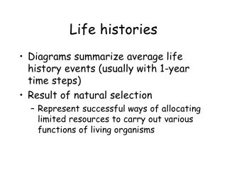
Life histories. Diagrams summarize average life history events (usually with 1-year time steps) Result of natural selection Represent successful ways of allocating limited resources to carry out various functions of living organisms. Tradeoffs. Size (survival) vs. number of offspring

E N D
Life histories • Diagrams summarize average life history events (usually with 1-year time steps) • Result of natural selection • Represent successful ways of allocating limited resources to carry out various functions of living organisms
Tradeoffs • Size (survival) vs. number of offspring • Fecundity vs. adult survival • Age at first reproduction • Fecundity and growth
Phenotypic plasticity: Solid line indicates that reaction norms can evolve! Figure 10.7
Environmental variation in biological conditions • Test for phenotypic plasticity by transplanting individuals (similar genotype) to several environments • Expose to predators, different resources
Membranipora membranacea: bryozoan common in the PNW Modular species: grows by making new feeding units at the edge of the colony. Chemicals released by predatory nudibranchs induce the formation of spines. Spines protect the bryozoan from predation by nudibranchs. Why not have them all the time?
Time to metamorphosis depends on food availability In this case, both time and size at metamorphosis are affected Figure 10.11
Phenotypic plasticity • Modular organisms can respond to environmental cues and alter the characteristics of new modules • Genotype x environment interaction: plasticity itself can adapt
Grime’s plant life histories • Competitive: Large, fast potential growth rate, early reproduction, vegetative spread • Ruderals: high potential growth rate, early reproduction, production is largely seeds, seed bank/ easily spread seeds • Stress tolerators: slow growth rate, late reproduction, little energy to seeds
These data show that plant species coexist best at low rates of fertilization, and moderate rates of disturbance in Minnesota prairies. • The authors suggest that coexistence is enhanced due to tradeoffs between competitive and colonization abilities. Wilson and Tilman 2002
Colonization ability (Seed dispersal) Competitive ability (Rate of nutrient use)
At low disturbance, lots of perennial plants, shrubs • At high disturbance, lots of annual plants, easily dispersed • But as soil is fertilized, competitive plants become more common throughout disturbance gradient Wilson and Tilman 2002
Populations:Distributions/ Life tables Ruesink lecture 4 Biology 356
Ecology includes the study of patterns in the distribution and abundance of species • Distribution is the spatial arrangement of organisms within a species • What is their total range? • Are there particular habitat associations? • Within a habitat, is the species clumped, random, or more evenly spaced?
Total species on earth Historical filter: Which taxa evolve? Physical filter: What is activity space? Biological filter: Effects of other species?
Figure 13.5 Three distinct ways that populations are distributed in space
Aspen: Clumped, random, or evenly spaced? Figure 13.7
Desert shrubs: Clumped, random, or evenly spaced? Figure 13.6
Distribution often depends on the scale of observation. How is this species distributed across its geographic range? How is it distributed within glades? How are individuals distributed within an aggregate? Figure 13.3
Ecology includes the study of patterns in the distribution and abundance of species • Abundance is the number of individuals in a population • Biologically, a population is a group of regularly-interbreeding individuals • Operationally, it is the size of the researcher’s study site
On average, every individual produces one successful offspring (replaces itself) • This case represents species that have populations in a dynamic steady state • Births equal deaths
Figure 14.12 Elephant seals: 1890 = 20; 1970 = 30,000
English ivy Scot’s broom Japanese oysters European starling
Invasive species • Non-indigenous = alien = exotic = introduced = non-native • Why (historically) aren’t all species everywhere? • Many species evolved in allopatry and have remained isolated by biogeographic barriers
Current rates of invasion are orders of magnitude higher than in the pastRuesink et al. 1995 Bioscience Cumulative number of species
In the Galapagos, number of alien plant species is closely related to the human population on the islands
Invasion pathways • Purposeful • Planned releases • Imports • Accidental
85% of exotic woody species in the U.S. were introduced for horticulture English holly English ivy Purple loosestrife European buckthorn
Costs and benefits • Estimated annual cost of invasive species in US = $137 billion based on 50,000 species ($41 B from crop weeds and pests) • Estimated annual benefits = crops and livestock • Pimentel et al. 2000 Bioscience
Population ecologyWhat makes a good invader? • Life history traits of successful invaders from first principles • High reproductive rate • Modular • Broad activity space = generalist, not specialist
Evidence – freshwater fishes with smaller body size are more likely to invade (shorter time to maturity)
Some species increase rapidly • Newly-introduced species • Species that can “outbreak” • Species hunted to low population levels and then protected • But sometimes they do not recover • Births exceed deaths
Is harvest or hydropower most responsible for the decline of Columbia River Chinook salmon? Kareiva et al. 2000
Runs in different seasons are genetically distinct Harvest Spawn and die Hatcheries Chinook spend 3-5 years in the ocean before returning Habitat Smolts migrate to estuary Hydropower
Some species are in decline • Most threatened and endangered species • Deaths exceed births
Ecologists have developed a simple (!) way of summarizing birth and death schedules • Follow the fate of one cohort through the lifespan OR Track the birth and death rates of each life stage
100 eggs Survive and grow to 25 tadpoles Survive and grow to 10 young frogs Survive and grow to 5 adult frogs, each of which lays 20 eggs
Survivorship 1.0 0.25 0.1 0.05 100 eggs Survive and grow to 25 tadpoles Survive and grow to 10 young frogs Survive and grow to 5 adult frogs, each of which lays 20 eggs
Mortality rate 0.75 0.6 0.5 ?? 100 eggs Survive and grow to 25 tadpoles Survive and grow to 10 young frogs Survive and grow to 5 adult frogs, each of which lays 20 eggs
Fecundity 0 0 0 20 100 eggs Survive and grow to 25 tadpoles Survive and grow to 10 young frogs Survive and grow to 5 adult frogs, each of which lays 20 eggs
Compare to life history diagram 20 0 1 2 3 0.4 0.5 0.25 Differences: Time steps need not be one year. All individuals move from current stage to the next.
Life tables • x = age • lx = survivorship up to age x (proportion living) • mx = mortality between age x and age x+1 • sx = survival rate from age x to age x+1 • bx = fecundity (births) at age x
Net reproductive rate • R0 • “R nought” • net reproductive rate, that is, number of offspring produced by average individual • R0 = S lx bx