Download
1 / 21
220 likes | 385 Views
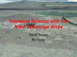
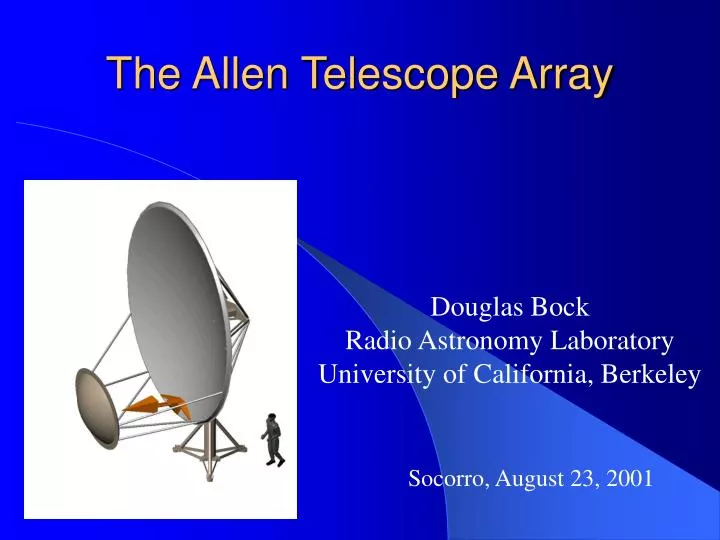
The Allen Telescope Array. Douglas Bock Radio Astronomy Laboratory University of California, Berkeley. Socorro, August 23, 2001. The Allen Telescope Array. Outline: System description Science goals Antenna configuration. ATA: What is It?. Massively parallel array of small dishes

E N D
The Allen Telescope Array Douglas BockRadio Astronomy LaboratoryUniversity of California, Berkeley Socorro, August 23, 2001
The Allen Telescope Array Outline: • System description • Science goals • Antenna configuration
ATA: What is It? • Massively parallel array of small dishes • 350 elements each 6.1 m in diameter • total collecting area larger than 100 m dish • 0.5 – 11.2 GHz simultaneously • multiple beams • Must be much cheaper than existing arrays • Joint project of SETI Institute and UC Berkeley • Funded by private donations • Access to the community determined by NSF contribution (but collaborative projects also possible)
IF Processing Tradeoffs to be made Likely to achieve # RF tunings (LO1’s) 4 # Beams (dual poln.) per RF tuning 4 BW per beam 100 MHz Constraints on beam locations primary beam? Image and alias rejection 30–40 dB Total of 16 dual polarization beams Only 5 K$ per antenna
Correlator • Image entire primary field of view • Large number of antennas is a challenge • Achievable BW will be set by funding • F/X design looks best for large N • Potential for using industry terabit switching • Likely 1024 channels in maximum BW 100 MHz
Beamformers Backends • Multiple beams speed up SETI searches • More than 1 star per field of view • Run in anticoincidence to identify RFI • Enables simultaneous SETI and radio astronomy • Pulsar research will be a major use • RA spectrometer in addition to correlator? • Active RFI suppression
ATA Performance Number of Elements 350 Element Diameter 6.10 m Total Geometric Area 1.02E+04 m^2 Aperture Efficiency 63% Effective Area 6.44E+03 m^2 2.33 K/Jy System Temperature 43 K System Eqiv. Flux Density 18 Jy Ae/Tsys 150 m^2/K Effective Array Diameter 687 m Natural Weighting Frequency 1 10 GHz Primary FoV 3.5 0.4 degree Synthesized Beam Size 108 11 arc sec Number of Beams >4 Continuum Sensitivity BW 0.2 GHz Confusion Flux Limit in 10 sec 0.41 mJy 0.1 mJy at 1.4 GHz Spectral Line Resolution 10 km/s Frequency 1 10 GHz BW 3.E+04 3.E+05 Hz Integration Time 1000 1000 sec RMS brightness 0.70 0.22 K
Unique features of the ATA • Wide field of view (2.5° @ 1.4 GHz) • Large-N design (N=350, D=6.1 m) • Broad instantaneous frequency coverage (0.5–11.2 GHz) • Ability to conduct several simultaneous observing programs
Key ATA science drivers • HI • All sky HI, z < 0.03, Milky Way at 100 s • 25% of northern sky to z ~ 0.2 • Zeeman • Magnetic Fields • Temporal Variables • Pulsar Timing Array • Pulsar survey follow-ups • Extreme Scattering Events • Transients • SETI • 100,000 FGK stars • Galactic plane survey (2nd generation DSP)
Configuration Requirements • SETI and pulsars/transients • low sidelobes • minimum shadowing • image southern sources • minimum confusion • Imaging projects — snapshots! • low sidelobes • sufficient resolution but good sensitivity to extended structure (for HI, best resolution which matches Tb sensitivity to z-sensitivity)
N Hat Creek Observatory 41° N, 121° W (Far northern California)
Optimizing uv Coverage • Fit uv coverage to a Gaussian model (F. Boone 2001a,b; A&A submitted and in prep.) • Model minimizes near sidelobes and forces a round beam (at chosen declination) • Maintains ‘complete’ uv coverage (to 440 m baselines) • Far sidelobes 1/N (rms)
Shadowing: 14% (2-hr, d = 29°) Filling factor: ~ 0.035
Nat. weighted beam 78 78 at d = 5° ( = 1.4 GHz) Sidelobes: near 0.9% peak; far 0.3% rms Contours: 0.3, 0.5, 0.9 … %
Shadowing: 18% (2-hr, d = 29°) Filling factor: ~ 0.035
Nat. weighted beam 78 78 at d = 23° ( = 1.4 GHz) Sidelobes: near 0.7% peak; far 0.3% rms Contours: 0.3, 0.5, 0.9 … %
Nat. weighted beam 78 78 at d = 23° ( = 1.4 GHz) Sidelobes: near 0.7% peak; far 0.3% rms Re-weight for rounder beam and sidelobes < 0.1% < 10% loss in sensitivity Truncate at Bmax = 440 m (limit of complete uv coverage) 84 beam, sidelobes 1.5% Put antennas in the road sidelobes 0.5% Lose 10% of antennas sidelobes 2% Random position error (1 m) no effect Contours: 0.3, 0.5, 0.9 … %
cf. the most compact configuration possible • Antennas within 280 m diameter (filling factor 0.15) [0.039] • Antennas still random (0.3% rms far sidelobes) • Uniform distribution (5% near sidelobes [0.7%]) • Transit beam 150 [78] • Shadowing 59% (2-hr, d = 29°) [18%]
2003-2004 Begin construction First use of partial array 2005 First hectare complete Feed into SKA technology decision point 1999-2001 R&D phase Rapid Prototyping Array Site selection Preliminary design reviews 2001-2002 Design phase Critical design reviews Production Test Array Plan construction phase Timeline for ATA