Download
1 / 12
120 likes | 259 Views
Regresión Lineal Simple. RS1. Plantas de Tratamiento de agua, DF , 1998. summary (modelo) Call : lm(formula = Vol ~ Cap ) Residuals : Min 1Q Median 3Q Max -1593.94 -188.53 -60.96 78.99 1212.30 Coefficients : Estimate Std . Error t value Pr(>|t|)

E N D
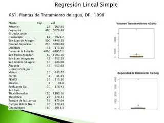
Regresión Lineal Simple RS1. Plantas de Tratamiento de agua, DF , 1998
summary(modelo) Call: lm(formula = Vol ~ Cap) Residuals: Min 1Q Median 3Q Max -1593.94 -188.53 -60.96 78.99 1212.30 Coefficients: EstimateStd. Error t value Pr(>|t|) (Intercept) 201.3821 126.8122 1.588 0.129 Cap 11.6783 0.1429 81.707 <2e-16 *** --- Signif. codes: 0 ‘***’ 0.001 ‘**’ 0.01 ‘*’ 0.05 ‘.’ 0.1 ‘ ’ 1 Residual standard error: 551.3 on 19 degrees of freedom Multiple R-squared: 0.9972, Adjusted R-squared: 0.997 F-statistic: 6676 on 1 and 19 DF, p-value: < 2.2e-16 anova(modelo) Analysis of Variance Table Response: Vol Df Sum Sq Mean Sq F value Pr(>F) Cap 1 2029113094 2029113094 6676.1 < 2.2e-16 *** Residuals 19 5774809 303937 Total 202034887903 --- Signif. codes: 0 ‘***’ 0.001 ‘**’ 0.01 ‘*’ 0.05 ‘.’ 0.1 ‘ ’ 1
shapiro.test(modelo$residual) Shapiro-Wilknormality test data: modelo$residual W = 0.8475, p-value =0.003846
Transformación de variable Analysis of Variance Table Response: y Df Sum Sq Mean Sq F value Pr(>F) Cap 1 36673 36673 184.94 3.047e-11 *** Residuals 19 3768 198 --- Signif. codes: 0 ‘***’ 0.001 ‘**’ 0.01 ‘*’ 0.05 ‘.’ 0.1 ‘ ’ 1 y<-sqrt(Vol) m2<-lm(y~Cap) Shapiro-Wilk normality test data: m2$residuals W = 0.9196, p-value = 0.08506
RS2. Modelo de Pinzones summary(m) Call: lm(formula = beak.length ~ mass, data = KenyaFinches) Residuals: Min 1Q Median 3Q Max -1.05373 -0.27044 -0.05373 0.33806 0.82956 Coefficients: EstimateStd. Error t value Pr(>|t|) (Intercept) 6.487159 0.112906 57.46 <2e-16 *** mass 0.110411 0.004608 23.96 <2e-16 *** --- Signif. codes: 0 ‘***’ 0.001 ‘**’ 0.01 ‘*’ 0.05 ‘.’ 0.1 ‘ ’ 1 Residual standard error: 0.4174 on 43 degrees of freedom Multiple R-squared: 0.9303, Adjusted R-squared: 0.9287 F-statistic: 574 on 1 and 43 DF, p-value: < 2.2e-16 > Schluter, D. 1988. The evolution of finch communities on islands and continents: Kenya vs. Galapagos. Ecological Monographs 58: 229-249.
anova(m) Analysis of VarianceTable Response: beak.length DfSumSq Mean Sq F value Pr(>F) Mass 1 100.000 100.000 574.03 < 2.2e-16 *** Residuals 43 7.491 0.174 Total 44 107.491 --- Signif. codes: 0 ‘***’ 0.001 ‘**’ 0.01 ‘*’ 0.05 ‘.’ 0.1 ‘ ’ 1 shapiro.test(m$residuals) Shapiro-Wilk normality test data: m$residuals W = 0.9784, p-value = 0.5572
RS3. Reforestación en el DF m<-lm(Reforestacion~Superfice) summary(m) Call: lm(formula = Reforestacion ~ Superfice) Residuals: Min 1Q Median 3Q Max -148.43 -97.75 -10.08 92.44 180.59 Coefficients: EstimateStd. Error t value Pr(>|t|) (Intercept) 186.3801 42.2576 4.411 0.000593 *** Superfice -0.3078 0.3439 -0.895 0.385911 --- Signif. codes: 0 ‘***’ 0.001 ‘**’ 0.01 ‘*’ 0.05 ‘.’ 0.1 ‘ ’ 1 Residual standard error: 111.4 on 14 degrees of freedomMultiple R-squared: 0.05412, Adjusted R-squared: -0.01344 F-statistic: 0.801 on 1 and 14 DF, p-value: 0.3859
anova(m) Analysis of Variance Table Response: Reforestacion Df Sum Sq Mean Sq F value Pr(>F) Superfice 1 9943 9943.1 0.801 0.3859 Residuals 14 173778 12412.7 Total 15 183721
RS4. Dióxido de Carbono por uso vehicular Año base 1970=100 Redfern, A., Bunyan, M., and Lawrence, T. (eds) (2003). The Environment in Your Pocket, 7thedn. London: UK Department for Environment, Food and Rural Affairs.
Call: lm(formula = co2 ~ uso) Residuals: Min 1Q Median 3Q Max -29.5946 -0.7761 1.0901 2.4873 6.8163 Coefficients: EstimateStd. Error t value Pr(>|t|) (Intercept) 25.39475 5.05584 5.023 3.16e-05 *** uso 0.75636 0.02999 25.223 < 2e-16 *** --- Signif. codes: 0 ‘***’ 0.001 ‘**’ 0.01 ‘*’ 0.05 ‘.’ 0.1 ‘ ’ 1 Residual standard error: 6.503 on 26 degrees of freedom Multiple R-squared: 0.9607, Adjusted R-squared: 0.9592 F-statistic: 636.2 on 1 and 26 DF, p-value: < 2.2e-16 Analysis of Variance Table Response: co2 Df Sum Sq Mean Sq F value Pr(>F) Uso 1 26904.1 26904.1 636.21 < 2.2e-16 *** Residuals 26 1099.5 42.3 Total 2728003.6 --- Signif. codes: 0 ‘***’ 0.001 ‘**’ 0.01 ‘*’ 0.05 ‘.’ 0.1 ‘ ’ 1