Download
1 / 43
430 likes | 594 Views
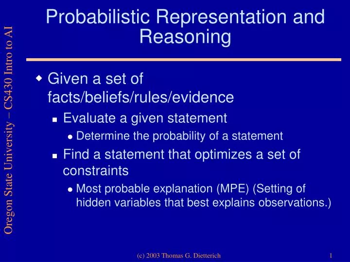
Probabilistic Representation and Reasoning. Given a set of facts/beliefs/rules/evidence Evaluate a given statement Determine the probability of a statement Find a statement that optimizes a set of constraints

E N D
Probabilistic Representation and Reasoning • Given a set of facts/beliefs/rules/evidence • Evaluate a given statement • Determine the probability of a statement • Find a statement that optimizes a set of constraints • Most probable explanation (MPE) (Setting of hidden variables that best explains observations.) (c) 2003 Thomas G. Dietterich
Probability Theory • Random Variables • Boolean: W1,2 (just like propositional logic). Two possible values {true, false} • Discrete: Weather 2 {sunny, cloudy, rainy, snow} • Continuous: Temperature 2< • Propositions • W1,2 = true, Weather = sunny, Temperature = 65 • These can be combined as in propositional logic (c) 2003 Thomas G. Dietterich
Example • Consider a car described by 3 random variables: • Gas 2 {true, false}: There is gas in the tank • Meter 2 {empty,full}: The gas gauge shows the tank is empty or full • Starts 2 {yes,no}: The car starts when you turn the key in the ignition (c) 2003 Thomas G. Dietterich
Joint Probability Distribution • Each row is called a “primitive event” • Rows are mutually exclusive and exhaustive • Corresponds to an “8-sided coin” with the indicated probabilities (c) 2003 Thomas G. Dietterich
Any Query Can Be Answered from the Joint Distribution • P(Gas = false Æ Meter = full Æ Starts = yes) = 0.0006 • P(Gas = false) = 0.2, this is the sum of all cells where Gas = false • In general: To compute P(Q), for any proposition Q, add up the probability in all cells where Q is true (c) 2003 Thomas G. Dietterich
Notations • P(G,M,S) denotes the entire joint distribution (In the book, P is boldface). It is a table or function that maps from G, M, and S to a probability. • P(true,empty,no) denotes a single probability value: P(Gas=true Æ Meter=empty Æ Starts=no) (c) 2003 Thomas G. Dietterich
Operations on Probability Tables (1) • Marginalization (“summing away”) • M,SP(G,M,S) = P(G) • P(G) is called a “marginal probability” distribution. It consists of two probabilities: (c) 2003 Thomas G. Dietterich
Conditional Probability • Suppose we observe that M=full. What is the probability that the car will start? • P(S=yes | M=full) • Definition: P(A|B) = P(A Æ B) / P(B) (c) 2003 Thomas G. Dietterich
Conditional Probability • Select cells that match the condition (M=full) • Delete remaining cells and M column • Renormalize the table to obtain P(S,G|M=full) • Sum away Gas: GP(S,G | M=full) = P(S|M=full) • Read answer from P(S=yes | M=full) cell (c) 2003 Thomas G. Dietterich
Operations on Probability Tables (2):Conditionalizing • Construct P(G,S | M) by normalizing the subtable corresponding to M=full and normalizing the subtable corresponding to M=empty (c) 2003 Thomas G. Dietterich
Chain Rule of Probability • P(A,B,C) = P(A|B,C) ¢ P(B|C) ¢ P(C) • Proof: (c) 2003 Thomas G. Dietterich
Chain Rule (2) • Holds for distributions too: P(A,B,C) = P(A | B,C) ¢P(B | C) ¢P(C) This means that for each setting of A,B, and C, we can substitute into the equation, and it is true. (c) 2003 Thomas G. Dietterich
Belief Networks (1):Independence • Defn: Two random variables X and Y are independent iff P(X,Y) = P(X) ¢P(Y) • Example: • X is a coin with P(X=heads) = 0.4 • Y is a coin with P(Y=heads) = 0.8 • Joint distribution: (c) 2003 Thomas G. Dietterich
Belief Networks (2)Conditional Independence • Defn: Two random variables X and Y are conditionally independent given Z iff P(X,Y | Z) = P(X|Z) ¢P(Y|Z) • Example: P(S,M | G) = P(S | G) ¢P(M | G) Intuition: G independently causes S and M (c) 2003 Thomas G. Dietterich
Operations on Probability Tables (3):Conformal Product • Allocate space for resulting table and then fill in each cell with the product of the corresponding cells: P(S,M | G) = P(S | G) ¢P(M | G) ¢ = (c) 2003 Thomas G. Dietterich
Properties of Conformal Products • Commutative • Associative • Work on normalized or unnormalized tables • Work on joint or conditional tables (c) 2003 Thomas G. Dietterich
Conditional Independence Allows Us to Simplify the Joint Distribution P(G,M,S) = P(M,S | G) ¢P(G) [chain rule] = P(M | G) ¢P(S | G) ¢P(G) [CI] (c) 2003 Thomas G. Dietterich
Bayesian Networks Gas • One node for each random variable • Each node stores a probability distribution P(node | parents(node)) • Only direct dependencies are shown • Joint distribution is conformal product of node distributions: P(G,M,S) = P(G) ¢P(M | G) ¢P(S | G) Meter Starts
Inference in Bayesian Networks • Suppose we observe that M=full. What is the probability that the car will start? • P(S=yes | M=full) • Before, we handled this by the following steps: • Remove all rows corresponding to M=empty • Normalize remaining rows to get P(S,G|M=full) • Sum over G: GP(S,G|M=full) = P(S | M=full) • Read answer from the S=yes entry in the table • We want to get the same result, but without constructing the joint distribution first. (c) 2003 Thomas G. Dietterich
Inference in Bayesian Networks (2) • Remove all rows corresponding to M=empty from all nodes • P(G) – unchanged • P(M | G) becomes P[G] • P(S | G) – unchanged • Sum over G: GP(G) ¢P[G] ¢P(S | G) • Normalize to get P(S|M=full) • Read answer from the S=yes entry in the table (c) 2003 Thomas G. Dietterich
Inference with Tables G (c) 2003 Thomas G. Dietterich
Inference with Tables G Step 1: Delete M=empty rows from all tables (c) 2003 Thomas G. Dietterich
Inference with Tables G Step 1: Delete M=empty rows from all tables Step 2: Perform algebra to push summation inwards (no-op in this case) (c) 2003 Thomas G. Dietterich
Inference with Tables G Step 1: Delete M=empty rows from all tables Step 2: Perform algebra to push summation inwards (no-op in this case) Step 3: Form conformal product (c) 2003 Thomas G. Dietterich
Inference with Tables Step 1: Delete M=empty rows from all tables Step 2: Perform algebra to push summation inwards (no-op in this case) Step 3: Form conformal product Step 4: Sum away G (c) 2003 Thomas G. Dietterich
Inference with Tables Step 1: Delete M=empty rows from all tables Step 2: Perform algebra to push summation inwards (no-op in this case) Step 3: Form conformal product Step 4: Sum away G Step 5: Normalize (c) 2003 Thomas G. Dietterich
Inference with Tables Step 1: Delete M=empty rows from all tables Step 2: Perform algebra to push summation inwards (no-op in this case) Step 3: Form conformal product Step 4: Sum away G Step 5: Normalize Step 6: Read answer from table: 0.6469 (c) 2003 Thomas G. Dietterich
Notes • We never created the joint distribution • Deleting the M=empty rows from the individual table followed by conformal product has the same effect as performing the conformal product first and then deleting the M=empty rows • Normalization can be postponed to the end (c) 2003 Thomas G. Dietterich
Cold Allergy Cat Sneeze Scratch Another Example: “Asia”(all variables Boolean) • Suppose we observe Sneeze • What is P(Cold | Sneeze) = P(Co|S)? (c) 2003 Thomas G. Dietterich
Answering the query • Joint distribution: A,Ca,ScP(Co) ¢P(A) ¢P(Sn | Co,A) ¢P(Ca) ¢P(A | Ca) ¢P(Sc | Ca) • Apply evidence: sn (Sneeze = true) A,Ca,ScP(Co) ¢P(A) ¢P[Co,A]¢P(Ca) ¢P(A | Ca) ¢P(Sc | Ca) • Push summations in as far as possible: • P(Co) ¢ AP(A) ¢P[Co,A] ¢CaP(A | Ca) ¢P(Ca) ¢ScP(Sc | Ca) • Evaluate: • P(Co) ¢ AP(A) ¢P[Co,A] ¢CaP(A | Ca) ¢P(Ca) ¢P[Ca] P(Co) ¢ AP(A) ¢P[Co,A] ¢P[A] P(Co) ¢ P[Co] P[Co] • Normalize and extract answer (c) 2003 Thomas G. Dietterich
Cold Allergy Cat Sneeze Scratch Pruning Leaves • Leaf nodes not involved in the evidence or the query can be pruned. • Example: Scratch Query Evidence (c) 2003 Thomas G. Dietterich
Greedy algorithm for choosing the elimination order nodes = set of tables (after evidence) V = variables to sum over while |nodes| > 1 do Generate all pairs of tables in nodes that share at least one variable Compute size of table that would result from conformal product of each pair (summing over as many variables in V as possible) Let (T1,T2) be the pair with smallest resulting size Delete T1 and T2 from nodes Add conformal product V T1¢T2 to nodes end (c) 2003 Thomas G. Dietterich
Example of Greedy Algorithm • Given tables P(Co), P[Co,A], P(A|Ca), P(Ca) • Variables to sum: A, Ca • Choose: P[A] = CaP(A|Ca) ¢P(Ca) (c) 2003 Thomas G. Dietterich
Example of Greedy Algorithm (2) • Given tables P(Co), P[Co,A], P[A] • Variables to sum: A • Choose: P[Co] = AP[Co,A] ¢P[A] (c) 2003 Thomas G. Dietterich
Example of Greedy Algorithm (3) • Given tables P(Co), P[Co] • Variables to sum: none • Choose: P2[Co] = P(Co) ¢P[Co] • Normalize and extract answer (c) 2003 Thomas G. Dietterich
… P1,1 P1,2 P2,1 P2,2 P1,3 P3,1 P1,4 … B1,1 B2,4 B1,3 B2,2 B3,1 B1,4 B2,3 B4,1 B1,2 B2,1 Bayesian Network For WUMPUS • P(P1,1,P1,2, …, P4,4, B1,1, B1,2, …, B4,4) (c) 2003 Thomas G. Dietterich
Probabilistic Inference in WUMPUS • Suppose we have observed • No breeze in 1,1 • Breeze in 1,2 and 2,1 • No pit in 1,1, 1,2, and 1,3 • What is the probability of a pit in 1,3? P(P1,3|:B1,1,B1,2,B2,1, :P1,1,:P1,2,:P2,1) (c) 2003 Thomas G. Dietterich
… P1,1 P1,2 P2,1 P2,2 P1,3 P3,1 P1,4 … B1,1 B2,4 B1,3 B2,2 B3,1 B1,4 B2,3 B4,1 B1,2 B2,1 What isP(P1,3|:B1,1,B1,2,B2,1, :P1,1,:P1,2,:P2,1)? false false query false false true true (c) 2003 Thomas G. Dietterich
… P1,1 P1,2 P2,1 P2,2 P1,3 P3,1 P1,4 … B1,1 B2,4 B1,3 B2,2 B3,1 B1,4 B2,3 B4,1 B1,2 B2,1 Prune Leaves Not Involved in Query or Evidence false false query false false true true (c) 2003 Thomas G. Dietterich
Prune Independent Nodes false false query false … P1,1 P1,2 P2,1 P2,2 P1,3 P3,1 P1,4 B1,1 B1,2 B2,1 false true true (c) 2003 Thomas G. Dietterich
Solve Remaining Network false false query false P1,1 P1,2 P2,1 P2,2 P1,3 P3,1 B1,1 B1,2 B2,1 P2,2,P3,1P(B1,1|P1,1,P1,2,P2,1) ¢P(B1,2|P1,1,P1,2,P1,3) ¢P(B2,1|P1,1,P2,1,P2,2,P3,1) ¢P(P1,1) ¢P(P1,2) ¢P(P2,1) ¢P(P2,2) ¢P(P1,3) ¢P(P3,1) false true true (c) 2003 Thomas G. Dietterich
Performing the Inference NORM{ P2,2,P3,1P(B1,1|P1,1,P1,2,P2,1) ¢P(B1,2|P1,1,P1,2,P1,3) ¢P(B2,1|P1,1,P2,1,P2,2,P3,1) ¢P(P1,1) ¢P(P1,2) ¢P(P2,1) ¢P(P2,2) ¢P(P1,3) ¢P(P3,1) } NORM{ P2,2,P3,1P[P1,3] ¢ P[P2,2,P3,1] ¢ P(P2,2) ¢ P(P1,3) ¢ P(P3,1) } NORM{ P[P1,3] ¢ P(P1,3) ¢ P2,2 P(P2,2) ¢ P3,1P[P2,2,P3,1] ¢P(P3,1) } P(P1,3) = h0.69, 0.31i 31% chance of WUMPUS! We have reduced the inference to a simple computation over 2x2 tables. (c) 2003 Thomas G. Dietterich
Summary • The Joint Distribution is analogous to the truth table for propositional logic. It exponentially large, but any query can be answered using it • Conditional independence allows us to factor the joint distribution using conformal products • Conditional independence relationships are conveniently visualized and encoded in a belief network DAG • Given evidence, we can reason efficiently by algebraic manipulation of the factored representation (c) 2003 Thomas G. Dietterich