Digital Testing: Role of Simulation in Testing

1. Digital Testing:Role of Simulation in Testing Based on text by S. Mourad "Priciples of Electronic Systems" and M. L. Bushnell and V. D. Agrawal, Essentials of Electronic Testing for Digital, Memory and Mixed-Signal VLSI Circuits

2. Outline • Verification and Simulation • Verification • Types of Simulation • Fault Simulation • Parallel Simulation • Concurrent Simulation • Deductive Simulation • Fault Coverage • Fault Dictionary

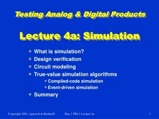
3. Types of simulation • Compiled simulator (table-driven) • Functional verification • Activity directed (event-driven)simulator • Event is a change in signal value • Useful for accurate timing models • Useful for asynchronous circuits

4. Types of Simulators • Logic versus Fault • Compiled versus event driven • Functional versus timing • Logic versus other levels (RTL or switch) • Mixed level • Emulators

5. Simulation of Large Systems • Explosion in number of gates used • Not possible with software to complete • Move to simulation of the whole circuit on • RTL level e.g. use of testbench in HDL • Cycle based Simulation • simulation of components at different levels using different simulator • relate the results using the same clock

6. Simulation System

7. Testbench: Example in Verilog ' timescale 1ns/1ns // Time unit is 1ns module adder; // Design Testbench reg PA, PB, PCI; wire PCO,PSUM; FA_Behav F1(PA, PB, PCI, PSUM,PCO);// Instantiate module undertest initial begin: ONLY_ONCE reg[3:0] Count; // Count hold the count of stimuli //4 bits are needed to accommodateup to 8. for (Count=0; Count < 8; PAL =Count +1) begin {PA, PB, PCI} =Count; //The stimuli are the values of Count #5 $display ("PA, PB, PCI=%b%b%b", PA, PB, PCI,":::PCO, PSUM=%b%b", PCO, PSUM); //Creation of the response display end end endmodule

8. Logic Simulation Verifies both function & timing Check that operation is : • independent on initial state • not sensitive to variations in delays • free of races, oscillations, illegal & hung-up states

9. Logic Simulation • Software Based • Slow • Hardware Accelerators • Simulation algorithm is hardwired • Improves performance with large set of inputs • Emulator • Prototyping and real time simulation • e.g. using FPGAs to implement the design • Pentium was emulated on 3500 Xilinx3000 FGPAs EPROM Emulator

10. Logic Simulation Levels Modeling level Function, behavior, RTL Logic Switch Timing Circuit Signal values 0, 1 0, 1, X and Z 0, 1 and X Analog voltage Analog voltage, current Application Architectural and functional verification Logic verification and test Logic verification Timing verification Digital timing and analog circuit verification Timing Clock boundary Zero-delay unit-delay, multiple- delay Zero-delay Fine-grain timing Continuous time Circuit description Programming language-like HDL Connectivity of Boolean gates, flip-flops and transistors Transistor size and connectivity, node capacitances Transistor technology data, connectivity, node capacitances Tech. Data, active/ passive component connectivity

11. Singular cover 0 1 X 0 0  0 1  1 1 X 0 1 X A cube of the Boolean function is a vector A simplified truth table based on singular cubes is called a singular cover Rules for intersection of cubes in Boolean logic

12. Exercise Check if the following cubes describe a logic function C1 1 1 x 0 C2 0 1 0 1 C3 0 x 1 1 C4 0 0 x 0

13. Exercise Check if the following cubes describe a logic function C1 1 1 x 0 C2 0 1 0 1 C3 0 x 1 1 C4 0 0 x 0 No, since 001 would cause 2 different output values as it belongs to both c3 and c4

14. 0 1 X U 0 0  0  1  1 1  X 0 1 X U U   U U Unknown logic value • Initial state of powered-up FF & RAMs is unpredictable • u -- denotes unknown logic value (0 or 1) • Boolean operation with u is a union of all operations on different values like OR(0,u)=OR{{0},{0,1}}={OR(0,0),OR(0,1)}={1,0}=u Intersection of cubes in 3 valued logic

16. 0 u u u u u 1 Pessimistic result in 3-valued simulation Since not(u) = u

17. Exercise Determine value of the logic function defined by the following cubes a) X10 0 b) 11X 0 c) X0X 1 d) 0 1 1 1 For the input vector I=(10u) using simulation

18. True-Value Simulation Algorithms • Compiled-code simulation • Applicable to zero-delay combinational logic • Also used for cycle-accurate synchronous sequential circuits for logic verification • Efficient for highly active circuits, but inefficient for low-activity circuits • High-level (e.g., C language) models can be used • Event-driven simulation • Only gates or modules with input events are evaluated (event means a signal change) • Delays can be accurately simulated for timing verification • Efficient for low-activity circuits • Can be extended for fault simulation

19. Compiled-Code Algorithm • Step 1: Levelize combinational logic and encode in a programming language • Step 2: Initialize internal state variables (flip-flops) • Step 3: For each input vector • Set primary input variables • Repeat (until steady-state or max. iterations) • Execute compiled code • Report or save computed variables

20. Levelization for Compiled Simulation

22. No more events Event-driven simulation flow Advance simulation time done Determine current events Update values Propagate events Evaluate activated elements Schedule resulting events

23. Delay models (a) Nominal transition-independent transport delay (b) Rise and fall delays (c) Ambiguous delay (d) Inertial delay (pulse suppression) (e) Output inertial delay

24. Delay models • Nominal transition-independent transport delay • (b) Rise and fall delays • (c) Ambiguous delay • (d) Inertial delay (minimum duration of input pulse) • (e) Output inertial delay A B=1 C A C C C C C 3 2 3 (a) d=2 (b) dr=1, df=3 (c) dm=1, dM=3 (d) dI = 4, (e) dI=2, d=3 1 5 R1 1 R2 3 3

25. A B C dI = 3 A B C 2 3 2 Output inertial delay The gate cannot produce impulse shorter than dI

26. Output inertial delay A B C dI = 3 A B C 2 2 1 3 3

27. Wire delays modeled by delay elements d1 d2

28. Element evaluation c i AND 0 0 OR 1 0 NAND 0 1 NOR 1 1 • Truth tables • quires 2n entries • Input Scanning • gates described by - c -- controlling value - i -- inversion c x x c  i x c x c  i x x c c  i c’ c’ c’ c’ i

29. Gate evaluation in 3-valued logic by scanning input values Evaluate (G, c, i) begin u_values = FALSE for every input value v of G begin if v = c then return c  i if v = u then u_values = TRUE end if u_values return u return c’  i end

30. Gate evaluation in 3-valued logic based on input counting evaluate (G, c, i) begin if c_count > 0 then return c  i if u_count > 0 then return u return c’  i end Advantage: No need to store the multiple input values (only two counters for c_count and u_count are updated during simulation) For instance in AND gate 1->0 change on its input increasesc_count while 0->u transition increases u_count and decreases c_count.

31. Hazard Detection A B Z Z A B R Q S Latch may be reset (Static hazard)

32. Unknown signal value B ==> B(t)B(t’)B(t+1) = 0u1 t t’ t+1 Also : A(t)A(t’)A(t+1) = 1u0 Z = (AB)’ = 1u1  {101, 111} -possible static hazard

33. Static Hazard Detection • Denote by E the set of inputs changing between t and t+1 • Procedure 3.1 • Set every input E to u and simulate to get output Z(t’) • Set every input E to its value at t+1 and simulate to get Z(t+1) • Theorem 3.1 • In a combinational circuit, a static hazard • exists iff Z(t)Z(t’)Z(t+1) is 1u1 or 0u0

34. C A B Hazard Detection Check the following circuit for static hazards If A = 010 then: (a) 0 delay : B = 101, C = 000 (b) unit delay : B = 1101, C = 0100 (c) arbitrary delay : A = 0u1u0, B = 1u0u1 => C = 0u0u0 (hazard)

35. Value Sequence(s) Meaning 0 000 Static 0 1 111 Static 1 0/1, R {001, 011} = 0u1 Rise (0 to 1) transition 1/0, F {110, 100} = 1u0 Fall (1 to 0) transition 0* {000, 010} = 0u0 Static 0-hazard 1* {111, 101} = 1u1 Static 1-hazard 6-valued logic for static hazard analysis

36. AND truth table for 6-valued logic

37. Dynamic Hazards • Dynamic hazards occur during transition • 1->0 or 0->1 • So they require 4 bit sequences to detect • 1010 or 0101 • To detect them in simulation 8 valued logic is used. • 8 valued logic can detect both static and dynamic hazards

38. 8-valued logic

39. Exercise To determine result of Boolean operation in 8 valued logic all possible sequences must be used For instance to calculate AND(R,1*) we have AND(R,1*)=AND({0x11,00x1},{1ux1,1xu1})= {0uu1,00u1}=R* Rules for inversion NOT(F)=R, NOT(0*)=1*, NOT(F*)=R*

40. R* F* 1 1 F* R* NAND 0 1 R F 0* 1* 0 1 1 1 1 1 1 1 1 0 F R 1* 0* R 1 F F 1* 1* F 1* 1* 1* F* R* F 1 R 1* R 1* R 0* 1 1* 1* 1* 1* 1* 1* 1 0* F R 1* 0* F* F* 1* 1* R* R* 1 F* 1* 1* F* 1 R* 1* R* NAND truth table for 8-valued logic Exercise: Calculate NAND(R,R*)

41. R* F* 1 1 F* R* NAND 0 1 R F 0* 1* 0 1 1 1 1 1 1 1 1 0 F R 1* 0* R 1 F F 1* 1* F 1* 1* 1* F* R* F 1 R 1* R 1* R 0* 1 1* 1* 1* 1* 1* 1* 1 0* F R 1* 0* F* F* 1* 1* R* R* 1 F* 1* 1* F* 1 R* 1* R* NAND truth table for 8-valued logic Exercise: Calculate NAND(R,R*) NAND(R,R*) = NAND({0x11,00x1},{0u01,01u1}) = NOT({0u01,01u1,0001,00u1}) = {1u10,10u0,1110,11u0}=F* Exercise: Calculate NAND(F,R*)

42. Event-Driven Procedure Event-Driven-Simulator: Read circuit description Read input vectors FOR each input vector to be simulated DO Process new inputs Update input nodes Schedule connected elements on timing wheel WHILE elements left for evaluation Evaluate element IF change on the output THEN update all fanouts and schedule Connect element on timing wheel END WHILE END FOR End procedure

43. A B Z Gate level event-driven simulation Only the activated gates are analyzed. Not all entries in the event list are events A B Z 0 2 4 6 8 10 12 8 10 12 (Z, 1) (Z, 0) (Z, 0) Not an event

44. Event Simulation While (event list not empty) begin t = next time in list process entries for time t end There is no events on G3, G5, G7, G8, and G9 due to F=1

45. max Current time pointer t=0 Event link-list 1 2 3 4 5 6 7 Time Wheel (Circular Stack)

46. i, vi’ j, vj’ * The Time Wheel Time in ns is computed modulo M  = tc mod M for events tc  te  tc + M-1 1   tc M If tc+ M  te then the event is put on the overflow queue

47. Event-Driven Algorithm(Example) Scheduled events c = 0 d = 1, e = 0 g = 0 f = 1 g = 1 Activity list d, e f, g g a =1 e =1 t = 0 1 2 3 4 5 6 7 8 2 c =1 0 g =1 2 2 d = 0 4 f =0 b =1 Time stack g 8 4 0 Time, t

48. A 7 12 20 25 B 5 10 25 35 C 2 12 20 30 35 C' 3 13 21 31 36 Delay d E A E 11 8 AND1 B F OR1 4 14 22 32 33 C' G F C INV G AND2 (b) XXXXXXXXXXXX D=1 E 12 16 (a) F XXXXXXXX 10 18 28 36 42 G XXXXXXXXXXXXX (c) 15 17 22 23 32 41 48 XXXXXXXXXXXXXX E 14 17 38 20 26 41 F XXXXXXXXXXXX 18 30 36 45 11 XXXXXXXXXXXXXXXXXXXX 26 30 45 G 37 40 22 (d) 24 Timing Simulation Unit delay Variable delay Rise and fall delay

49. Static Timing Simulation • Critical path delay • Using the circuit • and worst case analysis of delays • low complexity • Problems • No consideration for the function • False path

50. Oscillation Control When oscillation occur during simulation they waste simulator efforts – the same loops are traversed again and again • Local oscillation can be controlled by setting unstable feedback signals to u • Global oscillations are hard to control -- they are avoided by limiting the simulation time.