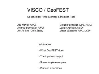
VISCO / GeoFEST Geophysical Finite Element Simulation Tool

1. VISCO / GeoFEST Geophysical Finite Element Simulation Tool Jay Parker (JPL) Andrea Donnellan (JPL) Jin-Fa Lee (Ohio State) Gregory Lyzenga (JPL, HMC) Louise Kellogg (UCD) Maggi Glasscoe (JPL, UCD) •Motivation • What GeoFEST does • The input and output • Some simple examples • Planned extensions

2. What GeoFEST does W G (G) • Volumetric: the volume is defined by space-filling tetrahedral elements • Displacement at nodes is the fundamental variable • Stress is a secondary property, computed for each element • Surface nodes carry special conditions • Can solve elastostatic problems as well as time-marching faulted VE

3. GeoFEST Features Geometry/Mesh Generation • Tied to unstructured mesh generator, mainly arb. rectangular patches • User specifies fault rectangles, material regions, mesh density Fault Physics • Periodic slip, or stress failure • Split-nodes store slip as evolving extra variable Rheology • Allows for layered, linear and power-law, elastic and viscoelastic materials Boundaries • Mix of fixed, free, surface tractions

4. Fundamental Equations Elastostatics: (leading toKu = f, instantaneous) Quasi-static Viscous: ("viscoplastic strain"; adds term to "f"; now Ku(t) = f(t); use implicit scheme of Hughes and Taylor ('78))

5. Motivation • LA basin has complex structure • Viscoelastic and poroelastic processes show up in geodetic data • Fault physics numerical laboratory

6. Input Categories • Nodes, their coordinates, fixed-or-free components, any imposed BC's • Elements, their material index and node list (volumetric and "fault") • Split nodes • Surface Tractions • Materials, their constituitive properties • Temporal variations: quake frequency, velocity BC changes, step control • Output control: report what, when • Misc: comments; smooth pressure? save functions? checkpoint? restart?

7. Input: what you need to specify • An output filename • random comments • Number of processors; how to divide nodes among processors (unsupported) • Number of displacement "freedoms": 3 for 3d; other options in 2D code • Number of time periods (0 for pure elastic; else governs steady epochs) • Flags for "save shape functions", "pressure smoothing" • Node freedom list • Node coords • Node imposed bc's: displacement, velocity • Volumetric properties for clusters of elts: type, integration rule, material • Element records (list of nodes, property id); supports a fault elt type, with properties • Split nodes • Surface tractions • Iteration limit and convergence criterion (unsupported) • Which node, element results to print out • Time step controls: # time groups, reform interval, when to save, when to break faults, group start times, implicit parameter, time step size • When to print outputs (list, or flag for "every quake") • (possible) restart file (i.e., start where another run left off, using this file) • (possible) save-state file (i.e., save this run so another run can start where we left off)

8. Outputs • Standard Out: comments, summary info, progress messages • Named output file: the requested node (displacement) and element (stress components), at the requested times • Restart file: contains "state" in ascii, but intended for machine reading

10. Example Runs • boxtest.dat (2D) • boxtest2.dat (2D) • block.mesh • block2.mesh • block3.mesh (piston) • block4.mesh (split) • "NR" meshes (elastostatic thrust fault in a box)

11. Block3: piston

12. "NR10" case using split nodes • Elastostatic: single "time step" solution • Or with viscous layers: maybe a few time steps in class time. • 23787 tetrahedral elements, 5395 nodes • 3944 split node records (node *and* element) elt node 0.5dx 0.5dy 0.5dz 1 5260 -0.15383 -0.48023 -0.41014 1 410 -0.15383 -0.48023 -0.41014 1 5343 -0.15383 -0.48023 -0.41014 2 5260 -0.15383 -0.48023 -0.41014 2 410 -0.15383 -0.48023 -0.41014 • • • Split nodes: special variable stores total screw dislocation Equivalent forces are applied to all surrounding nodes

13. Meshing methods 1) Paper, pencil, text editor (*small* meshes). 2) Above, plus refining tool like John Lou’s. 3) Clever perl scripts that lay out regular meshes (mkblock.prl). 4) Interactive graphics (RSI/IDL) tool for irregular 2D meshes. 5) Script wrappers around (research) 3D automeshing package. 6) Graphical interface around 3D automeshing. 7) Script wrappers around commercial 3D meshers. 8) Any of above plus regular refinement. 9) Any of above plus (research) adaptive refinement.

14. • Textual input for precision • Point/click for manipulation Interactive Graphics (2D)

15. Script wrappers around automeshing In some directory create file "params": number dip(o) strike(o) slip(m) rake(o) length(km) width(km) depth(km) 7 40.0 122 1.3 101 14.0 21.0 19.5 Run perl scripts 1) generate fault vertices, 2) generate domain 1) jimbo{jwp}245: ~jwp/src/gv/fault.prl NOTE: using fault parameters in file params Please supply meshing parameter on fault (km): 1.5 number dip(o) strike(o) slip(m) rake(o) length(km) width(km) depth(km) 7 40.0 122 1.3 101 14.0 21.0 19.5 hanging wall motion is 0.153834336428877 0.48023308511456 0.410135564047839 2) jimbo{jwp}246: ~jwp/src/gv/domain.prl Supply center (x,y), width (dx), length (dy), depth (dz), mesh parameter: 0 0 80 80 45 8 number dip(o) strike(o) slip(m) rake(o) length(km) width(km) depth(km) 7 40.0 122 1.3 101 14.0 21.0 19.5 Now you have cube.sld, fault.sld, and params in your directory: jimbo{jwp}265: cat fault.sld 4 20.3974 6.2236 -6.0015 8.5248 13.6425 -6.0015 0.0000 0.0000 -19.5000 11.8727 -7.4189 -19.5000 1 7 1 4 1 2 3 4 1.5 jimbo{jwp}264: cat cube.sld 8 -40.0000 40.0000 0.0000 40.0000 40.0000 0.0000 (etc) 6 1 1 4 1 2 3 4 8 2 1 4 5 6 7 8 8 (etc) Min element scale: use any editor to change, e.g. 4

16. Scripted automeshing (cont.) Create files cube.grp, cube.bcmap: jimbo{jwp}269: cat cube.grp 1.0 2 cube 1 0 8.0 fault 1 0 8.0 jimbo{jwp}270: cat cube.bcmap 7 1 1 (etc) 7 7 cube.grp, cube.bcmap, cube.sld, fault.sld: all you need to make a mesh! Now just issue the command (script invocation of automesher): mesh cube 0 This will create cube.node and cube.tetra. Now lee2vis.prl cube.node cube.tetra nr10.mesh will create "nr10.mesh"; ready to run with command geofest nr10.mesh

17. Graphical Interface Meshing • Project control and construction from parts database. • Can edit parts in widget windows. • Under adaptation to recognized geophysical terms. • Immediate check of gross errors. • Still relies on scripts for format conversion.

18. Linear Solvers • Note system is always positive definite. • Time steps use implicit technique, with matrix reform option. • Currently use node reordering and sequential Crout factorization. • Trial of ScaLAPACK banded solver underway. • Plans for parallel conjugate gradient using matrix slab partition.

19. Planned Extensions • Graphic feedback for geometry input • Adaptive meshing for error control • Better solver (preconditioned iterative), time-integrator • Faults with better motion conditions, e.g. slip-weakening, zero-strength • Better truncation boundaries, e.g., green's function expansion Note: GeoFEST volumetric formulation can also handle anisotropic materials with straightforward extension.

20. Conclusions • In-hand: volumetric finite element VE code GeoFEST -- periodic and stress-triggered faults -- interface to generation of unstructured mesh -- supports arbitrary faulting -- rheology may be quasi-static viscous, arbitrary geometry (e.g., blockwise-layered) • Planned expansions: --faulting physics (slip-weakening) --zero-strength faults --efficient solver/time stepping --smart domain-limiting boundaries --adaptive mesh --XML in/out, web-accessible object • Straightforward expansions: -- anisotropic rheology -- coupling via greens functions to far field, GEM