Download

1 / 32
330 likes | 518 Views
Chapter 8 Producers in the Long Run. Learning Objectives. 1. Discuss why profit maximization requires firms to equate the marginal product per dollar spent for all factors. (We skip this—saving it for intermediate micro.).

E N D
Chapter 8 Producers in the Long Run
Learning Objectives 1. Discuss why profit maximization requires firms to equate the marginal product per dollar spent for all factors. (We skip this—saving it for intermediate micro.) 2. Explain why firms will use more of the factors the prices of which have fallen, and less of the factors the prices of which have increased. 3. Describe the relationship between short-run and long-run cost curves. 4. Explain the importance of technological change and why firms are often motivated to innovate to improve their production methods. [We will skip this]
8.1The Long Run: No Fixed Factors In the short run, the only way to produce a given level of output is to adjust the input of the variable factors. In the long run, uses of ALL inputs are variable, and there are numerous ways to produce any given output. How does a firm choose how to produce? Two objectives: 1. Don’t waste society’s scarce resources, and 2. Produce the chosen output at least cost.
Technological Efficiency & Economic Efficiency • The decision of “how to produce” is made on the basis of what economists call “economic efficiency” –production at least cost • This is not the same as “technological efficiency,” but a process cannot be economically efficient unless it is also technologically efficient. • A process is technologically efficient if there is no other known way of producing • (a) the same output with less of at least one input and no more of any other, or equivalently • (b) more output using the same quantities of all inputs
Technological Efficiency • Three ways of producing 100 units of output • Method “A” uses same capital, less labour than “B” – “B” is not efficient (wastes resources) • Method “A” uses same labour, less capital than “C” – “C” is not efficient (wastes resources) • Method “A” dominates Methods “B” and “C”
When No Method is Dominated? • Technological efficiency is necessary for economic efficiency, but this criterion is not sufficient in all cases • If production takes place using more than a single input, there can be alternative input combinations (technologies) for producing the same output, none of which are dominated in a technological efficiency sense. • How would a firm choose in such a situation?
Three Methods of Producing 100 Units Method I Method II Method III 3 5 20 Capital Input 100 75 25 Labour Input How does the firm choose which method to use? What other information does the firm need?
Need Factor Prices, Compute Total Cost Method I Method II Method III 3 5 20 Capital Input 100 75 25 Labour Input 3*$100+100*$6 Price of Labour Price of Capital $100 $6 $900 $950 $2,150 $40 $10 $1,120 $950 $1,050 $30 $10 $1,090 $900 $850 3*$30 + 100*$10 20*$40 + 25*$10
Principle of Substitution Holding output constant, if it is possible to reduce total cost by substituting one factor for another, then the firm is not using the least costly combination of factors. The principle of substitution implies that a firm’s method of production will change if the relative prices of factors change. Relatively more of the cheaper factor and relatively less of the more expensive factor will be used. Substitution plays a central role in resource allocation because it describes how individual firms respond to changes in relative factor prices that are caused, in turn, by the changing scarcities of factors in the economy as a whole.
Long-Run Cost Curves When all factors of production can be varied, there exists a least average-cost method of producing any level of output. The long-run average cost (LRAC) curve is the boundary between cost levels that are attainable (with given technology and factor prices) and those that are unattainable... even when the use of ALL inputs (plant size, equipment, machinery [capital in general], as well as labour) can be varied by the firm. To illustrate…
Long-Run Cost Curves Consider production using various plant sizes or various amounts of machinery (amounts of capital). More capital means higher average and marginal product of labour (labour cost per unit of output falls), but… More capital means higher total fixed cost. For LOW rates of output, it makes little sense to use a lot of capital (very high average fixed cost), but... For HIGHER rates of output, fixed cost of larger amounts of capital can be spread (averaged) over more units, and Lower labour cost per unit (from higher labour productivity) outweighs the increase in fixed cost
Various Short-Run Total Cost Curves Cost ($/Unit) K1 < K2 < K3 < K4 < K5 TC-K5 TC-K4 TC-K3 TC-K2 TC-K1 Output per Period Use K1 Use K2 Use K3
Short-Run and Long-Run Average Cost Curves Cost ($/Unit) K1 < K2 < K3 < K4 < K5 SRAC-K1 SRAC-K5 SRAC-K4 SRAC-K2 SRAC-K3 LRAC Output per Period Use K1 Use K2 Use K3 Use K4 Use K5
Long-Run Average Cost Curve The Long Run Average Cost Curve serves to divide Attainable from Unattainable Levels of Cost (Can Do Worse, Cannot Do Better) Cost ($/Unit) Attainable (High) Levels of Cost LRAC Unattainable (Low) Levels of Cost Output per Period
SRATC2 Cost per Unit SRATC1 SRATC4 SRATC3 SRATC5 LRAC Output per Period No short-run cost curve can fall below the long-run curve because the LRAC curve shows the lowest attainable cost for each possible level of output. Each SRATC curve is tangent to the LRAC curve at the level of output for which the quantity of the fixed factor is optimal, and lies above it for all other levels of output. Note that the LRAC does NOT pass through the minimum point of a Short Run Average Cost if the tangency lies on the downward or upward sloping portion of LRAC
Long-Run Cost Curves Over the range from zero to qM, the firm has falling unit costs. This implies economies of scale (increasing returns to scale). Such a decreasing-cost firm is said to have increasing returns, which typically result from greater specialization made possible by the division of labour. Over the range from zero to qM to qD the firm has constant unit costs. This implies constant returns to scale. $/Unit LRAC Inc. Ret. to Sc. Const. Ret. to Sc. qD qM
Long-Run Cost Curves For output rates greater than qD the firm has rising unit costs. This implies diseconomies of scale (decreasing returns to scale). This typically results from difficulties in managing and controlling an enterprise as its size increases (increasing costs of control). $/Unit LRAC Inc. Ret. to Sc. Const. Ret. to Sc. Decr. Ret. to Sc. qD qM
Returns to Scale & LRAC What is it that is increasing, constant, or decreasing? Output per unit of (composite) input, certainly, but alsoprofit per unit FOR ANY FIXED PRICE, decreasing LRAC implies increasing profit per unit… constant LRAC implies constant profit per unit… increasing LRAC implies decreasing profit per unit. $/Unit LRAC P Inc. Ret. to Sc. Const. Ret. to Sc. Decr. Ret. to Sc. qD qM
Difference Between “Returns to Scale” and “Diminishing Marginal Product” • When the use of ALL inputs changes in the SAME proportion, we examine the resulting change in output • If the change in output is proportionally LESS than the change in the use of ALL inputs, we have decreasing returns to scale… • If the change in output is proportionally MORE than the change in the use of ALL inputs, we have increasing returns to scale… • “Returns to Scale” relates to the change in output that results from changing ALL inputs by the same proportion (multiplying by the SAME positive number)
Difference Between “Returns to Scale” and “Diminishing Marginal Product” • By contrast, “diminishing marginal product” refers to the change in output associated with changing the use of ONE input… holding the amounts of other input(s) FIXED • It is possible for a firm’s technology to exhibit increasing returns to scale at or around some level of output, while simultaneously experiencing diminishing marginal product of one input
“Returns to Scale” vs. “Diminishing Marginal Product” Over the range q1 to q2, the firm experiences increasing returns to scale (falling LRAC) if ALL inputs are increased in the same proportion. Over the same range q1 to q2, the firm experiences diminishing marginal product of the variable factor (labour), as shown by the rising SRAC-K1 curve FOR FIXED K = K1. Short run cost rises as output is increased to q2because K1 is the wrong amount of capital for producing q2 (should use K2 to minimize cost). Cost ($/Unit) SRAC-K1 SRAC-K2 LRAC q1 q2 Output per Period
“Returns to Scale” and LRAC Examples • If output increases by a SMALLER proportion than does input use, output increases at a Decreasing rate, and LRAC rises • If output increases by the SAME proportion as does input use, output increases at a Constant rate, and LRAC is unchanging (horizontal) • If output increases by a LARGER proportion than does input use, output increases at an Increasing rate, and LRAC falls
Decreasing Returns to Scale, Rising LRAC PC = r = $20PL = w = $10 Capital Used 1 4 9 9 16 16 25 Labour Used 1 4 4 9 16 25 25 Output 1 2 2.45 3 4 4.47 5 Capital Cost $20 $80 $180 $320 $500 Labour Cost $10 $40 $90 $160 $250 Total Cost $30 $120 $270 $480 $750 Average Cost $30 $60 $90 $120 $150 $/Unit 5 $150 Output Quantity 4 $120 LRAC 3 $90 2 $60 $30 1 5 10 15 20 25 1 2 3 4 5 Capital, Labour Output Quantity
“Returns to Scale” and LRAC Examples • If output increases by a SMALLER proportion than does input use, output increases at a Decreasing rate, and LRAC rises • If output increases by the SAME proportion as does input use, output increases at a Constant rate, and LRAC is unchanging (horizontal) • If output increases by a LARGER proportion than does input use, output increases at an Increasing rate, and LRAC falls
Constant Returns to Scale, Constant LRAC PC = r = $20PL = w = $10 Capital Used 1 4 9 9 16 16 25 Labour Used 1 4 4 9 16 25 25 Output 1 4 6 9 16 20 25 Capital Cost $20 $80 $180 $320 $500 Labour Cost $10 $40 $90 $160 $250 Total Cost $30 $120 $270 $480 $750 Average Cost $30 $30 $30 $30 $30 $/Unit 25 $50 Output Quantity 20 $40 LRAC 15 $30 10 $20 $10 5 5 10 15 20 25 5 10 15 20 25 Capital, Labour Output Quantity
“Returns to Scale” and LRAC Examples • If output increases by a SMALLER proportion than does input use, output increases at a Decreasing rate, and LRAC rises • If output increases by the SAME proportion as does input use, output increases at a Constant rate, and LRAC is unchanging (horizontal) • If output increases by a LARGER proportion than does input use, output increases at an Increasing rate, and LRAC falls
Increasing Returns to Scale, Falling LRAC PC = r = $20PL = w = $10 Capital Used 1 2 3 3 4 4 5 Labour Used 1 2 2 3 4 5 5 Output 1 4 9 27 256 1024 3125 Capital Cost $20 $40 $60 $80 $100 Labour Cost $10 $20 $30 $40 $50 Total Cost $30 $60 $90 $120 $150 Average Cost $30 $15 $3.33 $0.47 $0.05 $/Unit 250 $15 Output Quantity 200 $12 150 $9 100 $6 LRAC $3 50 1 2 3 4 5 50 100 150 200 250 Capital, Labour Output Quantity
To recap: • falling LRAC ==> increasing returns to scale; • constant LRAC ==> constant returns to scale; • rising LRAC ==> decreasing returns to scale.
Efficient Scale, MINIMUM Efficient Scale, Capacity Any output level that can be produced at the LOWEST Long Run Average Cost is characterized as an Efficient Scale of output. If there is a range over which the firm experiences Constant Returns to Scale (the Long Run Average Cost is constant)… and if, over that range, the LRAC is at its minimum, then there are many output levels satisfying the definition of Efficient Scale The SMALLEST of these flow rates of output at which the firm attains minimum LRAC is called the firm’s MinimumEfficient Scale of output.
Minimum Efficient Scale The SMALLEST of these flow rates of output at which the firm attains minimum LRAC is called the firm’s MinimumEfficient Scale of output. $/Unit Efficient Scale Output Rates LRAC Minimum Efficient Scale qMES Output per Period
Shifts in LRAC Curves We saw in Chapter 7 how changes in either technology or factor prices cause the entire family of short-run costs curves to shift. The same is true for long-run cost curves. A rise in factor prices shifts short-run and long-run average cost curves upward. A fall in factor prices or a technological improvement shifts short-run and long-run average cost curves downward.