Download
1 / 46
640 likes | 1.45k Views
Chap 2 Introduction to Statistics. This chapter gives overview of statistics including histogram construction, measures of central tendency, and dispersion. INTRODUCTION TO STATISTICS. Statistics – deriving relevant information from data Deals with

E N D
Chap 2 Introduction to Statistics This chapter gives overview of statistics including histogram construction, measures of central tendency, and dispersion
INTRODUCTION TO STATISTICS • Statistics – deriving relevant information from data • Deals with • Collection of data – census, GDP, football, accident, no. of employees (male, female , department, etc) • Collection , tabulation, analysis, interpretation, an presentation of quantitative data – can make some conclusions on sample or population studied, make decisions on quality
INTRODUCTION TO STATISTICS • Use of statistics in quality deals with second meaning. – inductive statistics • Examples : • What can we learn from the data? • What conclusions can be drawn? • What does the data tell about our process and product performance? etc.
INTRODUCTION TO STATISTICS • Understand the use of statistics vital in business • to make decisions based on facts • in conducting business improvements • in controlling and monitoring process, products or service performance • Application of statistics to real life problems such as for quality problems will result in improved organizational performance
Collection of data • Collect Data – direct observation or indirect through written or verbal questions (market research, opinion polls) • Direct observation measured, visual checking, classified as variables and attributes • Variables data – measurable quality characteristics • Attributes – characteristics not measured but classified as conforming or non-conforming
Collection of data • Data collected with purpose • Find out process conditions • For improvement • Variables – quality characteristics that are measurable and countable • CONTINUOUS - Dimensions, weight, height, etc. (meter, gallon, p.s.i., etc.) • DISCRETE - numbers that exhibit gaps, countable, (no. of defective parts, no. of defects/car, Whole numbers, 1, 2, 3….100)
Collection of data • Attributes - quality characteristics that are non-measurable and ‘those we do not want to measure’ • Example : surface appearance, color, Acceptable, non-acceptable conforming, non-conf. • Data collected in form of discrete values • Variables (weight of sugar) CAN be classified as attributes • weight within limits – number of conforming • outside limits – no. of non conforming
Summarizing Data • Consider this data set on number of Daily Billing errors • Data in this from • Meaningless • Not effective • Difficult to use
Need to summarize data in the form of: • Graphical – Freq. Dist., Histogram, Graphs, Charts, Diagrams • Analytical – Measures of central tendency, Measure of dispersion
Frequency Distribution (FD) • Summary of how data (observations) occur within each subdivision or groups of observed values • Help visualize distribution of data • Can see how total frequency is distributed • Two types : • Ungrouped data – listing of observed values • Grouped data – lump together observed values
FD - Ungrouped Data • Establish array, arrange in ascending or descend (as in column 1) • Tabulate the frequency – place tally marking in column 2 • Present in graphical form – Histogram, Relative freq. distr.
14 12 10 8 6 4 2 0 4 1 2 3 5 FD – Ungrouped data • 4 graphical representations • Frequency histogram • Relative freq histogram • Cumulative frequency histogram • Relative cum frequency histogram Frequency
Frequency Distribution For Grouped Data • Data which are continuous variable need grouping Steps 1. Collect data and construct tally sheet • Make tally - coded if necessary • Too many data – group into cells • Simplify presentation of distribution • Too many cells – distort true picture • Too few cells – too concentrated • No of cells – judgment by analyst – trial and error • Generally 5-20 cells • Less than 100 data – use 5 –9 cells • 100 – 500 data – use 8 to 17 cells • More than 500 – use 15 to 20 cells
Cell interval (i) CELL Midpoint UPPER BOUNDARY CELL NOMENCLATURE
2. Determine the range • R = XH - XL • R = range • XH = highest value of data • XL = lowest value of data • Example : • If highest number is 2.575 and lowest number is 2.531, then • R = XH - XL • = 2.575 – 2.531 • = 0.044
3. Determine the cell interval • Cell interval = distance between adjacent cell midpoints. If possible, use odd interval values e.g. 0.001, 0.07, 0.5 , 3; so that midpoint values will have same no. decimal places as data values. • Use Sturgis rule. • i = R/(1+ 3.322 log n) • Trial and error • h = R/i ;h= number of cells or cllases • Assume i = 0.003; h = 0.044/0.003 = 15 cells • Assume i = 0.005; h = 0.044/0.005 = 9 cells • Assume ii = 0.007; h = 0.044/0/.007 = 6 cells • Cell interval 0.005 with 9 cells will give best presentation of data. Use guidelines in step 1.
2.533 2.538 4. Determine cell midpoints • MPL = XL + i/2 (do not round) • = 2.531 + 0.005/2 = 2.533 • 1st cell have 5 different values (also the other cells) 2.531 2.532 2.533 2.534 2.535
5. Determine cell boundaries • Limit values of cell • lower • upper • To avoid ambiguity in putting data • Boundary values have an extra decimal place or sig. figure in accuracy that observed values • + 0.0005 to highest value in cell • - 0.0005 to lowest value in cell
6. Tabulate cell frequency • Post amount of numbers in each cell • Frequency distribution table
Freq dist gives better view of central value and how data dispersed than the unorganized data sheet • Histogram – describes variation in process • Used to • solve problems • determine process capability • compare with specifications • suggest shape of distribution • indicate data discrepancies, e.g. gaps
Sym. Skew Right Skew Left Bi-modal flatter platykurtic ‘very peak’ leptokurtic Characteristics Of Frequency Distribution • Symmetry, Number of modes (one, two or multiple), Peakedness of data
Characteristics of Frequency Distribution • F.D. can give sufficient info to provide basis for decision making. • Distributions are compared regarding:- Shape Spread Location
Descriptive Statistics • Analytical method allow comparison between data • 2 main analytical methods for describing data • Measures of central tendency • Measures of dispersion • Measures of central tendency of a distribution - a numerical value that describes the central position of data • 3 common measures • mean • median • mode
Measure of Central Tendency • Mean - most common measure used • What is middle value? What is average number of rejects, errors, dimension of product? • Mean for Ungrouped Data - unarranged • x (x bar)
Mean Example A QA engineer inspects 5 pieces of a tyre’s thread depth (mm). What is the mean thread depth? x1 = 12.3 x2 = 12.5 X3 = 12.0. x4 = 13.0 x5 = 12.8
Mean - Grouped Data • When data already grouped in frequency distribution fi (n)= sum. of freq. fi = freq in the ith cell n = no. of cells/class xi = mid point in ith cell
Mean - Grouped Data = 2700/50 = 54
Weighted average Tensile tests aluminium alloy conducted with different number of samples each time. Results are as follows: 1st test : x1 = 207 MPa n = 5 2nd test : x2 = 203 MPa n = 6 3rd test : x3 = 206 MPa n = 3 or use sum of weights equals 1.00 W1 = 5/(5+6+3) = 0.36 W2 = 6/(5+6+3) = 0.43 W3 = 3/(5+6+3) = 0.21 Total = 1.00 xw = weighted avg. wi = weight of ith average
Median – Ungrouped Data • Median – value of data which divides total observation into 2 equal parts • Ungrouped data – 2 possibilities • When total number of data (N) is a) odd or b) even • If N is odd ; (N+1/2)th value is median • eg. 3 4 5 6 8 N+1/2=6/2=3 , 3rd no. • If N is even • eg. 3 5 7 9 ½ of (5+7)=6 • NOTE: ORDER THE NUMBERS FIRST!
Median – Grouped Data • Need to find cell / class having middle value & interpolating in the cell using Lm = lower boundary of cell with the median Cfm = Cum. freq. of all cells below Lm fm =class/cell freq. where median occurs i = cell interval Example MD = 40.5 + 10 = 53.5
Measures of dispersion • describes how the data are spread out or scattered on each side of central value • both measures of central tendency & dispersion needed to describe data • Exams Results • Class 1 – avg. : 60.0 marks • highest : 95 • lowest : 25 • Class 2 – avg. : 60.0 marks • highest : 100 • lowest : 15 marks
Measures of dispersion • Main types – range, standard deviation, and variance • Range – difference bet. highest & lowest value • R = XH - XL • Standard deviation • Variance – standard deviation squared • Large value shows greater variability or spread
Standard deviation • For Ungrouped Data • s = sample std. dev. xi = observed value x = average n = no. of observed value • or use
Standard deviation – grouped data NOTE: DO NOT ROUND OFF fixi & fixi2 ACCURACY AFFECTED
Concept Of Population and Sample • Total daily prod. of steel shaft. • Year’s Prod. Volume of calculators • Compute x and s sample statistics • True Population Parameters • and • Why sample? • not possible measure population • costs involved • 100% manual inspection – accuracy/error Population Sample
POPN. Parameter - mean - std. dev. SAMPLE Statistics, x , s Concept Of Population and Sample
ND Normal Distribution • Also called Gaussian distribution • Symmetrical, unimodal, bell-shaped dist with mean, median, mode same value • Popn. curve – as sample size cell interval - get smooth polygon
Normal Distribution • Much of variation in nature & industry follow N.D. • Variation in height of humans, weight of elephants, casting weights, size piston ring • Electrical properties, material – tensile strength, etc.
Characteristics of ND • Can have different mean but same standard deviation
Normal Distribution Example • Need estimates of mean and standard deviation and the Normal Table • Example : • From past experience a manufacturer concludes that the burnout time of a particular light bulb follows a normal distribution. Sample has been tested and the average (x ) found to be 60 days with a standard deviation () of 20 days. How many bulbs can be expected to be still working after 100 days.
Solution • Problem is actually to find area under the curve beyond 100 days • Sketch Normal distribution and shade the area needed • Calculate z value corresponding to x value using formula • Z=(xi - )/ = (100-60)/20 = +2.00 • Look in the Normal Table for z = +2.00 – gives area under curve as 0.9773 • But, we want x >100 or z > 2.00. Therefore Area = 1.000 – 0.9773 = 0.0227, i.e. 2.27% probability that life of light bulb is > 100 hours σ =20 μ = 60 0 100 x
Test For Normality • To determine whether data is normal • Probability Plot - plot data on normal probability paper • Steps • Order the data • Rank the observations • Calculate the plotting position i= rank , n=sample size, PP= plotting position in % • Label data scale • Plot the points on normal probability paper • Attempt to fit by eye ‘best line’ • Determine normality