Games as adversarial search problems
130 likes | 248 Views
This document explores adversarial search in dynamic game environments, focusing on the Minimax algorithm and its application in two-player turn-taking zero-sum games. It delves into how state spaces are structured, with variables defining game conditions and the role of transition edges in legal moves. The importance of the evaluation function for strategic decision-making is emphasized, alongside the challenges posed by extensive state spaces. The content is insightful for those studying computer science, artificial intelligence, or game theory.

Games as adversarial search problems
E N D
Presentation Transcript
Games as adversarialsearch problems Dynamic state space search
Requirements ofadversarial game space search • on-line search: planning cannot be completed before action • multi-agent environment • dynamic environment D Goforth - COSC 4117, fall 2003
Features of games King’s Court • deterministic/stochastic • perfect/partial information • number of agents: n>1 • optimization function • interaction scheduling • deterministic • perfect • 2 • zero-sum • turn-taking D Goforth - COSC 4117, fall 2003
Games as state spaces • state space variables describe relevant features of game • start state(s) define initial conditions for play • any legal state of the game is a state in the space • transition edges in the space define legal moves by players • two player turn-taking games define bi-partite state spaces • terminal states (no out-edges) are determined by a ‘terminal test’ and define end-of-game D Goforth - COSC 4117, fall 2003
Example game: • turn-taking zero-sum game: • two players: Max (plays first), Min • n tokens • rules: take 1, 2 or 3 tokens • start state: 5 tokens, Max to play • goal: take last token D Goforth - COSC 4117, fall 2003
Example game: state space Turn Max Min Max Min Max 5 4 3 2 3 2 1 2 1 0 1 0 2 1 0 1 0 0 1 0 0 0 1 0 0 0 0 0 State: (number of tokens remaining, whose turn) e.g., (2,Max) D Goforth - COSC 4117, fall 2003
Example game: Max’s preferences Turn Max Min Max Min Max 5 4 3 2 - - 3 2 1 2 1 0 1 0 + + + + + + 2 1 0 1 0 0 1 0 0 0 - - - - 1 0 0 0 0 + 0 evaluation function for Max: + for win (0, Min), - for loss at terminal state (0, Max) D Goforth - COSC 4117, fall 2003
Example game: Max’s move, why? Turn Max Min Max Min Max 5 - - + 4 3 2 - - + + + + + + 3 2 1 2 1 0 1 0 - - - - + + + + + + 2 1 0 1 0 0 1 0 0 0 - - - - + 1 0 0 0 0 + 0 see p.166, Fig. 6.3 Minimaxback propagation of terminal states assumption: opponent (Min) is also smart D Goforth - COSC 4117, fall 2003
Minimax algorithm • Back propagation in dynamic environment • evaluate state space to decide one move • attempt to find move that is best for all possible reactions • Minimax assumption • worst case assumption about dynamic aspect of environment (opponent’s choice) • if assumption wrong, situation is better than assumed D Goforth - COSC 4117, fall 2003
Minimax algorithm • Deterministic if • environment is deterministic (no random factors) • Exhaustive search to terminal states - time complexity is O(bm) b: number of moves in a game m: number of actions per move e.g. chess b 50, m 20, bm 1033 D Goforth - COSC 4117, fall 2003
Minimax search ininteresting games • space is too large to search to terminal states (except possibly in endgames) • use of heuristic functions to evaluate partial paths • deeper search evaluates ‘closer’ to terminal states D Goforth - COSC 4117, fall 2003
Minimax in large state space maximization minimization heuristic evaluation from viewpoint of Max D Goforth - COSC 4117, fall 2003
The search-evaluate tradeoff • branching factor n • execution time for heuristic evaluation t • search to level k • total time: nkt = nk-1(nt) to go a level deeper in same time, evaluation function must be n times more efficient • special situations: start game, end game D Goforth - COSC 4117, fall 2003