Download
1 / 30
300 likes | 389 Views
Analyzing the SEVIRI Precipitating Clouds Product and its performance using different algorithms, spectral features, and cloud microphysics. Results show the likelihood of precipitation with intensity classifications.

E N D
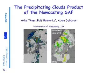
The SEVIRI Precipitating Clouds Product of the Nowcasting SAF: First results 15 October 2004 IPWG-2, Monterey Anke Thoss Swedish Meteorological and Hydrological Institute Ralf Bennartz University of Wisconsin
Contents • Introduction • Algorithm • Examples • Performance • Plans
Problem overview: • Except for strong convection, VIS/IR features are not • strongly correlated with precipitation. likelihood estimates in intensity classes more appropriate than rain rate retrieval NWCSAF approach: 2 complementary products for Nowcasting purposes Precipitating Clouds (PC) product gives likelihood of precipitation in coarse intensity classes 2. Convective Rain Rate (CRR) product estimates rain rate for strongly convective situations
PC product: three classes of precipitation intensity from co-located radar data Rain rate Class 0: Precipitation-free 0.0 - 0.1 mm/h Class 1: Light/moderate precipitation 0.1 - 5.0 mm/h Class 2: Intensive precipitation 5.0 - ... mm/h
Data sets for algorithm development Colocated sets of: AVHRR NWP Tsurface (HIRLAM) radar reflectivities (dBZ), gauge adjusted, of the BALTRAD Radar Data Centre BRDC (Michelsson et.al. 2000) No quantitative tuning to MSG performed for version 1.0 which is presented here!
Input: • NWCSAF Cloud type product • NWP surface temperature (ECMWF) • MSG channels : 0.6 m, 1.6 m, 3.9 m, 11 m and 12 m
Algorithm development: • Based on Cloud type output • Correlation of spectral features with precipitation investigated • Special attention to cloud microphysics (day/night algorithms) • Precipitation Index PI constructed as linear combination of spectral features • Algorithms cloud type specific
Correlation of Spectral features with rain Correlation with class, all potentially raining cloudtypes T11 -0.24 Tsurf - T11 0.26 T11-T11 -0.16 R0.6 0.18 R3.7 -0.18 ln(R0.6/R3.7) 0.26 R0.6/R1.6 0.42 3.7mday algorithm, all 0.35 1.6m day algorithm, all 0.44 night algorithm, all 0.30
Probability distribution, all raining Cloudtypes Night algorithm 3.7 Day algorithm 1.6 Day algorithm
Precipitation Index Example AVHRR 3.7 day algorithm, all cloud types: PI=35+0.644(Tsurf-T11)+5.99(ln(R0.7/R3.7))-3.93(T11-T12) Example AVHRR 1.6 day algorithm, all cloud types: PI = 65 -15*abs(4.45-R0.6 /R1.6)+0.495*R0.6-0.915(T11-T12) +0*Tsurf+0*T11 MSG day algorithm: Blend of 3.7µm day algorithm (applied to 3.9 µm channel) and 1.6 µm algorithm with equal weight, some additional features introduced for later use in quantitative tuning (a8-a10): PI=a0 +a1*Tsurf +a2*T11+a3*ln(R0.6/R3.9)+a4*(T11-T12) +a5*abs(a6-R0.6/R1.6)+a7*R0.6 + a8*R1.6+a9*R3.9+a10*(R1.6/R3.9) MSG night algorithm still identical to PPS
100% - 70% 60% 50% 40% 30% 20% 10% 0% Cloud type and total precipitation likelihood (day), March 2004, 12UTC
Night algorithm, courtesy of M. Putsay, Hungarian Meteorological Service
05:30 06:30 07:30 Upper:PC1, lower:PC2, 20031014
30 min. sampling 10 min. sampling
high+ very high opaque medium level Cirrus moderate-thick Ci over lower cloud
20% POD= 0.76 FAR= 0.73 PODF= 0.16 HK= 0.60 BIAS= 2.85 ACC= 0.84 30% POD= 0.58 FAR= 0.65 PODF= 0.08 HK= 0.50 BIAS= 1.66 ACC= 0.89 20% POD= 0.78 FAR= 0.81 PODF= 0.17 HK= 0.61 BIAS= 4.13 ACC= 0.83 30% POD= 0.62 FAR= 0.74 PODF= 0.09 HK= 0.52 BIAS= 2.42 ACC= 0.89 20% likelihood threshold N=36466 Rain: 7.1% (30min) 4.9% (10min)
20% likelihood threshold N=36466 Rain: 7.1% (30min) 4.9% (10min) Percent of total number Percent of gauge class
MSG PC Product validation with surface observations • Dataset: 15 May – 18 June 2004 12:00 UT: • MSG data and • Collocated surface observations of present weather (only ww classes indicating clearly rain or no rain considered) • PC product without use of cloud type (only a NN based cloud mask)
Validation of MSG PC product • Day, 45 N – 55 N, Total data points : 12123 (4.6 % raining) • Likelihood of precipitation agrees well with synop
Validation of MSG PC product • Night, 45 N – 55 N, Total data points : 12123 (4.6 % raining) • Likelihood of precipitation agrees well with synop
Validation of MSG PC product • Day, 30 N – 45 N, Total data points : 7218 (2.5% raining) • Likelihood of precipitation is over-estimated by the PC product
Validation of MSG PC product • Night, 30 N – 45 N, Total data points : 7218 (2.5 % raining) • Likelihood of rain is over-estimated by the PC product
20% POD= 0.90 FAR= 0.78 PODF= 0.16 HK= 0.74 BIAS= 4.12 ACC= 0.84 20% POD= 0.88 FAR= 0.78 PODF= 0.16 HK= 0.72 BIAS= 4.17 ACC= 0.84 20% likelihood threshold N=12123 4.6% raining
20% POD= 0.92 FAR= 0.84 PODF= 0.13 HK= 0.79 BIAS= 5.78 ACC= 0.86 20% POD= 0.91 FAR= 0.86 PODF= 0.14 HK= 0.77 BIAS= 6.51 ACC= 0.86 20% likelihood threshold N=7218 2.5% raining
Why does verification against SYNOP WW look better than for gauge comparison (POD)? (parallax adjustment, alg0 better than alg1-alg4, May/June easier, all difficult ww excluded …) Timescale / horizontal scale (real effect or convenient Bias correction?) How can false alarms be reduced further? Open questions
Algorithm Performance – Summary Night algorithm seems OK for strong convection, but overestimates precipitation (extent and intensity) for frontal situations Day algorithm better in general, but has no skill to class precipitation intensity recommended to display total precipitation likelihood Discontinueties between day and night algorithm Precipitation likelihood fairly correct between 45-55N South of 45N precipitation likelihood overestimated
What is next? tuning against European synop, covering a years cycle Status: ongoing while tuning, try to decrease discontinuaty between day and night algorithm, especially for PC2 need more gauge data for PC2 tuning later: investigate usefulness of additional channels