Download
1 / 24
240 likes | 416 Views
Linear Algebra on GPUs. Jens Krüger Technische Universität München. Linear algebra?. Why are we interested in Linear Algebra? It is THE machinery to solve PDEs PDEs are at the core of many graphics applications Physics based simulation, Animation, Mesh fairing …. LA on GPUs?.

E N D
Linear Algebra on GPUs Jens Krüger Technische Universität München
Linear algebra? • Why are we interested in Linear Algebra? It is THE machinery to solve PDEs • PDEs are at the core of many graphics applications Physics based simulation, Animation, Mesh fairing …
LA on GPUs? • … and why put LA on GPU? A perfect couple… GPUs are fast stream processors, and many LA operations are “streamable” …which goes hand in hand The solution is already on the GPU and ready for display
Visual simulation Visual computing Education and Training Basic linearalgebra operators General linear algebra package Highbandwidth Parallelcomputing Getting started … Computer graphics applications GPU as workhorse for numerical computations Programmable GPUs
Visual simulation Visual computing Education and Training Basic linearalgebra operators General linear algebra package Highbandwidth Parallelcomputing Getting started … Computer graphics applications GPU as workhorse for numerical computations Programmable GPUs
1 N 1 N Internal affairs • Per-pixel vs. per-vertex operations • 6 gigapixels/second vs. 0.7 gigavertices/second • Efficient texture memory cache • Texture read-write access • 2D Textures are even better • 2D RGBA textures really rock • Textures best we can do Vector representation
N Vectors Matrix i N 2D-Textures 1 i N ... ... ... ... N N N N 1 i Representation (cont.) Dense Matrix representation • Treat a dense matrix as a set of column vectors • Again, store these vectors as 2D textures
2 Vectors i 2 2D-Textures 1 2 N N N-i 1 2 Representation (cont.) Banded Sparse Matrix representation • Treat a banded matrix as a set of diagonal vectors • Combine opposing vectors to save space Matrix N
Vector 1 Vector 2 Pass through TexUnit 0 TexUnit 1 Vector 3 return tex0+tex1 Operations 1 • Vector-Vector Operations • Reduced to 2D texture operations • Coded in pixel shaders • Example: Vector1 + Vector2 Vector3 Render Texture Static quad Vertex Shader Pixel Shader
st nd 1 pass 2 pass original Texture ... ... ... ... Operations 2 (reduce) Reduce operation for scalar products Reduce m x n region in fragment shader
The “single float” on GPUs Some operations generate single float values e.g. reduce Read-back to main-mem is slow Keep single floats on the GPU as 1x1 textures ...
N Vectors Matrix i 2 Vectors Matrix i N 2D-Textures 1 i N ... ... ... ... N 2 2D-Textures N N 1 2 N-i N N N N 1 i 1 2 Operations (cont.) Matrix-Vector Operations • Split it up into Vector – Vector operations
Operations In depth example: Vector / Banded-Matrix Multiplication A b x =
Example (cont.) Vector / Banded-Matrix Multiplication A b A b x =
= Example (cont.) Compute the result in 2 Passes: A Pass 2 Pass 1 b x b‘
Building a Framework Presented so far: • Representations on the GPU for • Single float values • Vectors • Matrices • Dense • Banded • Random sparse (see SIGGRAPH ‘03) • Operations on these representations • Add, multiply, reduce, … • Upload, download, clear, clone, …
Framework Example: CG Encapsulate into Classes for more complex algorithms • Example use: Conjugate Gradient Method, complete source: voidclCGSolver::solveInit() { Matrix->matrixVectorOp(CL_SUB,X,B,R); // R = A*x-b R->multiply(-1); // R = -R R->clone(P); // P = R R->reduceAdd(R, Rho); // rho = sum(R*R); } voidclCGSolver::solveIteration() { Matrix->matrixVectorOp(CL_NULL,P,NULL,Q); // Q = Ap; P->reduceAdd(Q,Temp); // temp = sum(P*Q); Rho->div(Temp,Alpha); // alpha = rho/temp; X->addVector(P,X,1,Alpha); // X = X + alpha*P R->subtractVector(Q,R,1,Alpha); // R = R - alpha*Q R->reduceAdd(R,NewRho); // newrho = sum(R*R); NewRho->divZ(Rho,Beta); // beta = newrho/rho R->addVector(P,P,1,Beta); // P = R+beta*P; clFloat *temp; temp=NewRho; NewRho=Rho; Rho=temp; // swap rho and newrho pointers } void clCGSolver::solve(intmaxI) { solveInit(); for (inti = 0;i< maxI;i++) solveIteration(); } intclCGSolver::solve(floatrhoTresh,intmaxI) { solveInit(); Rho->clone(NewRho); for (inti = 0;i< maxI && NewRho.getData() > rhoTresh;i++) solveIteration(); returni; }
Example 12D Waves (explicit) • Finite difference discretization: • You could write a custom shader for this filter • Think about this as a matrix-vector operation
2D Waves (cont.) One Time Matrix Initialization: for (i=sY;i<sX*sY;i++) data[i] = ß; // setup diagonal-sY matrix->getRow(sX*(sY-1))->setData(data); for (i=0;i<sX*sY;i++) data[i] = (i%sX) ? ß : 0; // setup diagonal-1 matrix->getRow(sX*sY-1)->setData(data); for (i=0;i<sX*sY;i++) data[i] = 2-4ß; // setup diagonal matrix->getRow(sX*sY)->setData(data); for (i=0;i<sX*sY;i++) data[i] = ((i+1)%sX) ? ß : 0; // setup diagonal+1 matrix->getRow(sX*sY+1)->setData(data); for (i=0;i<sX*(sY-1);i++) data[i] = ß;// setup diagonal+sY matrix->getRow(sX*(sY+1))->setData(data); Per Frame Iteration clMatrix->matrixVectorOp(CL_SUB,clCurrent,clLast,clNext); // next = matrix*current-last; clLast->copyVector(clCurrent); // save for next iteration clCurrent->copyVector(clNext); // save for next iteration cluNext->unpack(clNext); // unpack for rendering renderHF(cluNext->m_pVectorTexture); // render as heightfield
+ t 1 t x c - 4+1 - 1 1 + t 1 t x c - - - 4+1 2 2 + t t 1 c x - - 4+1 3 3 + t t 1 x c - - 4+1 - 4 4 = + t t 1 c x - - - - 4+1 5 5 + t t 1 c x - - 4+1 - 6 6 + t t 1 c x - - 4+1 7 7 + t t 1 c x - - 4+1 - 8 7 + t t 1 c x - - 4+1 9 9 Example 22D Waves (implicit) Key Idea • Use different time discretization (e.g. Crank Nicholson) • Results in system of linear equations • Iterative solution using CG
2D Waves (cont.) One Time Matrix Initialization: for (i=sY;i<sX*sY;i++) data[i] = -alpha; // setup diagonal-sY matrix->getRow(sX*(sY-1))->setData(data); for (i=0;i<sX*sY;i++) data[i] = (i%sX) ? - alpha : 0; // setup diagonal-1 matrix->getRow(sX*sY-1)->setData(data); for (i=0;i<sX*sY;i++) data[i] = 4*alpha+1 // setup diagonal matrix->getRow(sX*sY)->setData(data); for (i=0;i<sX*sY;i++) data[i] = ((i+1)%sX) ? -alpha:0; // setup diagonal+1 matrix->getRow(sX*sY+1)->setData(data); for (i=0;i<sX*(sY-1);i++) data[i] = -alpha // setup diagonal+sY matrix->getRow(sX*(sY+1))->setData(data); Per Frame Iteration cluRHS->computeRHS(cluLast, cluCurrent); // generate c(i,j,t) clRHS->repack(cluRHS); // encode into RGBA iSteps = pCGSolver->solve(iMaxSteps); // solve using CG cluLast->copyVector(cluCurrent); // save for next iteration clNext->unpack(cluCurrent); // unpack for rendering renderHF(cluCurrent->m_pVectorTexture); // render as heightfield
The End Thank you! Questions? For more infos, browse to: http://wwwcg.in.tum.de/GPU http://www.gpgpu.org