Download
1 / 50
500 likes | 604 Views
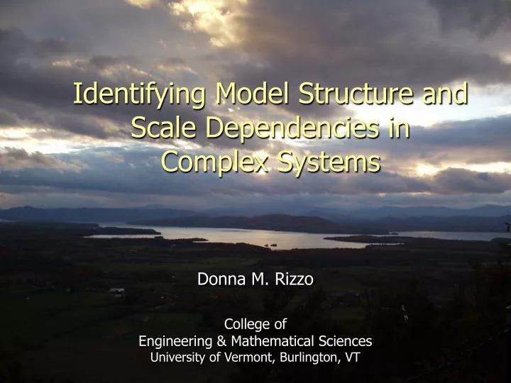
Identifying Model Structure and Scale Dependencies in Complex Systems . Donna M. Rizzo College of Engineering & Mathematical Sciences University of Vermont, Burlington, VT . Minimize = Real $$$ + l * (Performance & Resource Targets). N. N. p. w. å. å. =. +. +. ). q. F. N. F.

E N D
Identifying Model Structure and Scale Dependencies in Complex Systems Donna M. Rizzo College of Engineering & Mathematical Sciences University of Vermont, Burlington, VT
Minimize = Real $$$+l * (Performance & Resource Targets) N N p w å å = + + ) q F N F f ( l C , C , W,T “The extrapolations are the only things that have any real value. … Knowledge is of no real value if all you can tell me is what happened yesterday….you must be willing to stick your neck out.” i treat w cap MCL = = 1 1 k i R. P. Feynmann,The Uncertainty of Science, John Danz Lecture, April 23, 1963 Forecast Modeling & Heuristic Optimization Methods
Mass Remaining and Cost Cost ($ 10M) Mass (Mg) Performance-Cost “Ratio” Time (years) Time (years) l = 1 l = 5 l = 10 Multi-objective Optimization Rizzo and Dougherty, Water Resources Research, 30 (2), pp. 483-497, 1994. Which scheme is “optimal” ? - How long do we really have to operate? - How long do we really have to monitor? - How much residual risk are we willing to accept? - Will a new technology or public policy shift become available?
Conclusions • There’s no such thing as “correct scale”… (it’s problem dependent) • Keys: - recognizing when a change in scale has occurred - determining what information (and what scale) data must be collected
Geostatsitics • Variogram – Estimate of Correlation in Space • Range • Distance where samples are no longer correlated • Sill • Variance where samples are no longer correlated • Ordinary Kriging • Spatial Estimation at unknown locations
Initial C (ppb), Jan., 1998 Kriged, July, 1999 HGL Model, July, 1999 Bayesian, July, 1999 Combining Geostatistics with Process Modeling
Figure 5. General positive relationship between MWIBI (Mixed Water Index of Biotic Integrity) and patch-ordered rank. Clark, Rizzo, Watzin, and Hession, River Research and Applications, 23, DOI: 10.1002/rra.1085, 2007.
Parameter Estimation Application: Estimation of Berea Sandstone Geophysical Properties Lance Besaw
Berea Sandstone Data Data collected by New England Research, Inc. (see Boinott, G. N., G. Y. Bussod, et al., 2004. "Physically Based Upscaling of Heterogeneous Porous Media: An Illustrated Example Using Berea Sandstone." The Leading Edge.
Z Direction (mm) X Direction (mm) Sample Dataset • Exhaustive Dataset: All measurements (3800) • Sample Dataset (limited number of data): • Primary data (air permeability) known at screened elevations (46 measurements). • Secondary data (compressional-wave velocity & electrical resistivity) known along 10 well borings (380 measurements).
Single Neuron V1 V2 . . . VN W1 W2 . . . WN f(Sp) Σ vi wip = sp Y Sp Artificial Neural Networks (ANNs) • Data driven, real-time prediction • Large amounts of multiple data types • Parallel processing • Non-parametric statistics (few data assumptions) Inputs Weights Activation Function Output
Counterpropagation Algorithm • Supervised neural network • Combines • 1. Kohonen Self-organizing map (unsupervised NN) • 2. Grossberg outstar structure (operates as a Bayesian classifier) • Self-organizes in response to examples of some function (training data) • Training phase • Network learns inherent relationships within data • Prediction/implementation phase • Extracted inherent relationships are utilized
Hidden Layer Output Layer (Kohonen) (Grossberg) Input Layer x Estimate Air permeability along well borings z . . . . . . . . . . . . Restivity . . . . . . P-Velocity Estimating Air Permeability
Hidden Layer Output Layer (Kohonen) (Grossberg) Input Layer x Estimate Air permeability everywhere within the domain z . . . . . . . . . . . . . . . . . . Estimating Air Permeability
Sandstone Air Permeability Air Permeability Omnidirectional Variogram 15000 Semi-Variogram Bin Averages 95% Confidence Limit 10000 (permeability) 5000 g 0 0 50 100 150 200 250 300 350 Cokriged Estimates of Permeability Distance (mm) Ordinary Cokriging Permeability Estimates ANN Estimates of Permeability Geostatistics (Cokriging) Estimate Field Besaw and Rizzo, Water Resources Research, 43, W11409, DOI: 10.1029/2006WR005509, 2007.
Improving site characterization & monitoring environmental change using microbial profiles and geochemistry in landfill-leachate contaminated groundwater Cassella Waste Services Schuyler Landfill, N.Y. Department of Civil & Environmental Engineering Bernie Nadeau Donna Rizzo Paula Mouser Department of Biology Department of Geology Greg Druschel Patrick O’Grady Lori Stevens Brooke Schwartz
Long Term Monitoring Challenges at Landfills • What do you monitor in landfill leachate? • What are the monitoring objectives? • Monitoring for how long and at what frequency?
Motivation Microbial diversity can be leveraged between clean and contaminated environments.
PCA - Hydrochemistry • Contaminated Locations Separate Across PC1 • Fringe Locations Not Separated Across PC1-PC3 • 60% Variance Explained in first 2 PCs • PC1 Correlations • TDS, Mg, Cl, Spec Cond, Hardness, Alkalinity, COD, TOC, NH3 • PC2 Correlations • Organic-N, Phenols
PCA - All Data • Clean, Fringe, and Contaminated Locations Separated in PC1-PC2 • 22% Variance Explained • PC1 Correlations • TDS, Mg, Spec Cond, Alkalinity, Na, Cl, Hardness, COD, TOC, NH3, Eh, Mn, SO4 • G505, B244, B122, G80, B168, G165, A244 • PC2 Correlations • Fe, NO3, pH • B121, B160, G424, A118, G510, A144, B492, G484, B279, B470
Delineating contamination at landfill sites without prior knowledge Mouser, Rizzo, Röling, and van Breukelen, Environmental Science & Technology, 39 (19) pp. 7551-7559, 2005.
Motivation Mouser, Rizzo, Röling, and van Breukelen, Environmental Science & Technology, 39 (19) pp. 7551-7559, 2005.
A Modified Self-Organizing Map for Spatial Clustering Andrea Pearce
Kohonen self-organizing map • Non parametric clustering algorithm - useful when groupings unknown • Unsupervised ANN • Usages: complex non-linear mappings, data compression, clustering • Disparate data types • Used in ecological studies to model benthic macro invertebrates in streams Park et al. (2003) and Gevreyet al.(2004)
The Self-Organizing Map 6 features per sampling location 25 sampling locations Output Space 2D Map Small W(i,j,1) W(i,j,2) Medium W(i,j,3) Big W(i,j,4) 2-legs The algorithm finds the best matching node on the output map… W(i,j,5) W(i,j,6) 4-legs Hair
The Self-Organizing Map 6 features per sampling location 25 sampling locations Output Space 2D Map Small W(i,j,1) W(i,j,2) Medium W(i,j,3) Big W(i,j,4) 2-legs …and updates weights in the neighborhood of that node. W(i,j,5) W(i,j,6) 4-legs Hair
Kohonen’s Animal Example Unified Distance Matrix (U-Matrix)
Kohonen’s Animal Example Component Planes
Cyanobacteria Blooms and Cyanotoxin Production • We will cluster samples based on cyanobacterial communities using a Self-Organizing Map (SOM) • Then compare the clusters to measured cyanotoxin concentrations www.lcbp.org A bloom near Venise-en-Quebec in August, 2008. Credit: Quebec Ministry of Sustainable Development, Environment and Parks.
Advances in Watershed Management and Fluvial Hazard Mitigation Using Artificial NeuralNetworks and Remote Sensing Lance Besaw1, Donna M. Rizzo1, Michael Kline3, Kristen Underwood4, Leslie Morrissey2 and Keith Pelletier2 1College of Engineering and Mathematics, University of Vermont, Burlington, VT 2Rubenstein School of Natural Resources,University of Vermont, Burlington, VT 3River Management Program, Vermont Agency of Natural Resources, Waterbury, VT 4South Mountain Research & Consulting, Bristol, VT
Stressors Leading toChannel Instability • Increased hydraulic loading (climatic and % impervious) • Increased sediment loads • Channelization / Straightening • Floodplain encroachment • Loss of riparian buffer • Channel Armoring • Undersized bridges / culverts (constriction) • Instability resulting from multiple (natural and human) stressors causes stream to move out of dynamic equilibrium. • The State of Vermont wants to make reasonable predictions of instability.
Vermont Agency of Natural ResourcesRiver Management Program • Channel and watershed management • Channel dynamic equilibrium • Avoid infrastructure disasters • State wide data collection • Expert assessments • Fluvial erosion hazard mapping • Stakeholder Planning Tool • Data driven, translate to multiple geographic locations • GIS-based for visualization, quantification, communication, prioritization • Incorporate process-based classification of river networks • Real-time, multiple-objective management decisions • http://www.anr.state.vt.us/dec/waterq/rivers.htm
State Wide Stream Assessments • Phase 1 – watershed and channel corridor features • Land cover/use • Sinuosity • Channel slope • Geologic soils, etc • Phase 2 - Field assessment • Incision ratio • Access to flood plain • Grain size distribution, etc • Rapid geomorphic assessment (RGA)
Stream Sensitivity • Likelihood of stream adjustment in response to watershed or local stressors fluvial erosion hazard ratings, water quality, habitat indices • Based on… • Inherent vulnerability – hydraulic geometry and sediment regime • Geomorphic condition– degree of departure from dynamic equilibrium (or reference condition) • Based on research findings from Lane (1955), Schumm (1977), Knighton (1988), Rosgen (1996), Simon and Thorne (1996), Montgomery and Buffington (1997), MacBroom (1998) and others.
Inherent Vulnerability (g) Stream Sensitivity SOM Width/depth ratio Sinuosity Slope … Channel material … … … Impervious area Riparian vegetation Stream Sensitivity GeomorphicCondition Degradation Aggradation Widening … Planform Change Hierarchical ANNs for Stream Sensitivity Single/multiple threads Entrenchment ratio
Remote Sensing – Sensitivity Analysis • Light Detection and Ranging (LIDAR) • Aid land use/land cover classifications • More accurately compute • Valley width • Channel/valley slope • Definiens eCognition – object based classifier • Classify Sinuosity • Incorporate LIDAR for land use/land cover classification
Geomorphic Condition Over-Widening Degradation / Incision Planform Change Aggradation
Reach - level Input RGA score quartile Condition Code (VTDEC, 2002) Poor 1 1 to 5 Fair 2 6 to 10 Good 3 11 to 15 Optimal 4 16 to 20 Geomorphic Condition ANN Inputs • Rapid Geomorphic Assessment:ranks dominant process of adjustment (degradation, aggradation, widening, and planform change) and stage of channel evolution http://www.anr.state.vt.us/dec/waterq/rivers.htm
y y Geomorphic Condition 0.4 0.1 0.3 0.2 0 1 0 0 0 1 0 0 15 12 9 14 Output Pattern Output Pattern Target Pattern Predicting Geomorphic Condition Scores Adjust internal weights Channel Degradation Channel Aggradation Channel Widening Planform Change Input Layer Hidden Layer Output Layer Input Pattern
Geomorphic Condition ANN: Example Burlington Lewis Creek Middlebury River
Geomorphic Condition ANN Results R2 = 0.854
Single/multiple channel(s) Entrenchment ratio Inherent Vulnerability Width/depth ratio Sinuosity Slope … Channel material Inherent Vulnerability ANN(Combined Rosgen and Montgomery & Buffington) • Trained to be Quality Assurance look-up table • Predict stream inherent vulnerability on 789 VT reaches • Prediction Accuracy • 80% classification agreement with recorded field data • 12% due to imprecise parameter boundaries (overlap) • 8% due to data transfer mistakes (or additional expert knowledge)
Hierarchical ANNs for Stream Sensitivity Inherent Vulnerability Single/multiple threads Entrenchment ratio (g) Stream Sensitivity SOM Width/depth ratio Sinuosity Slope … Channel material … … … Impervious area Riparian vegetation GeomorphicCondition Degradation Aggradation Widening … Planform Change
Hierarchical ANNs for Stream Sensitivity • Predicting Stream Sensitivity (789 reaches) • 75% classification agreement • 22% differ by 1 class • 3% differ by >1 class
Kohonen hidden nodes Low & Very Low Moderate ic High High Nc High Very High & Extreme Very High Extreme Self-organizing map Input nodes Inputs Inherent Vulnerability Geomorphic Condition
Conclusions • ANNs are data-driven (flexible and simple to modify enabling a truly adaptive management approach) • Can be modified to recognize when a change in scale has occurred • Process of training - elicits significance of governing factors in determination of sensitivity- helps document similarities/differences among experts (and weighting of parameters for classifying vulnerability, condition, and overall sensitivity
Acknowledgements • VT Agency of Natural Resources, River Management Program • USGS • NSF EPSCoR Graduate Research Assistantship • Evan Fitzgerald; School of Natural Resources, University of Vermont, Burlington, VT • Jeff Doris; Sanborn, Head and Associates, Randolph, VT Questions
References • Gevrey, M., Rimet, F., Park, Y. S., Giraudel, J.-L., Ector, L., and Lek, S. (2004). "Water quality assessment using diatom assemblages and advanced modelling techniques." Freshwater Biology, 49, 208-220. • Kohonen, T. (1989). Self-Organization and Associative Memory, Springer Verlag, New York. • Lane, E.W. (1955) “The importance of fluvial morphology in hydraulic engineering.” Proceedings of the Ammerican Society of Civil Engineers, Journal of the Hydraulics Division, (81), paper no. 745. • Montgomery, D. R. and Buffington, J. M. (1997) “Channel-reach morphology in mountain drainage basins.” Geological Society of America Bulletin, 109(5), 596-611. • Park, Y.-S., Cereghino, R., Compin, A., and Lek, S. (2003). "Applications of artificial neural networks for patterning and predicting aquatic insect species richness in running waters." Ecological Modelling, 160, 265-280. • Rosgen, D. L. (1996) Applied Fluvial Morphology, Wildland Hydrology, Pasoda Springs, CO. • Schumm, S. A. (1977) The Fluvial System, John Wiley and Sons, New York, NY.