Understanding Labor Demand and Profit Maximization in Economics
90 likes | 216 Views
This analysis explores the factors affecting labor demand in the context of profit maximization and competition. It discusses how changes in wages, worker productivity, and the number of firms influence labor demand. The demand for labor is shown to be derived fromproduct demand, with a focus on the principles of marginal revenue and costs. The role of firms as price-takers in perfect competition is evaluated alongside the significance of marginal productivity in labor and capital inputs. Understanding these dynamics is crucial for comprehending production decisions in the short run.

Understanding Labor Demand and Profit Maximization in Economics
E N D
Presentation Transcript
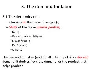
3. The demand for labor 3.1 The determinants: • Changes on the curve wages (-) • Shifts of the curve (ceteris paribus): • DC (+) • Workers productivity (+) • No. of firms (+) • PK, Pi (+ or -) • Other… The demand for labor (and for all other inputs) is a derived demand–it derives from the demand for the product that helps produce
3.2 Profit maximization • Main assumption behind the DL profit max. • Classical assumption firms are “price-takers” • Perfect competition • Decisions on production (what, how, how much) • DL stems from marginal changes • Decision flow output level and optimal mix of inputs • Incremental decisions how long?
3.2 Profit maximization • Maximizing firm expand output…insofar as MR > MC YC up • When will output be diminished? MR < MC YC down • Equilibrium MR = MC YC constant • For ΔYC Δ inputs (L, K) In terms of inputs: MRPL > MWC L up MRPL < MWC L down MRPL = MWC L constant profit maximization
3.2 Profit maximization • This flow of decisions will determine how to increase or diminish production marginally • Therefore, whenever we employ 1 additional unit of L (or K), we will generate additional income for the output produced and sold • So, the MRPL is the multiplication of two terms: • Δ output (MPL) • Δ revenue for the additional unit of output, produced and sold (unit MRPL)
3.2 Profit maximization Some definitions: • MPL = ΔY/ΔL; with K fixed • MPK = ΔY/ΔK; with L fixed • unit MRPL depends on market conditions • Equal to price of perfect competition (“price-takers”) • MRPL = MPL x unit MRPL also = MPL x P (in PC) • MRPK = MPK x unit MRPK also = MPK x P (in PC)
3.3 Demand in the short run: perfect competition (product market) The “short run” assumption allows us to treat K as fixed PFSR = YSR= f ( L, K ) In the short run, decisions by the firm regarding output and labor input are two sides of the same coin The only thing that matters in the short run is whether the output level should be altered (we know how to do it: with L)
3.3 Demand in the short run: perfect competition (product market) What can be deduced from the production function? MPL = ΔY/ΔL APL = Y/L The relationships between Y, MPL, & APL are important When MPL > APL APL is growing Production function (zones): 1) Y grows, growing rate (MPL & APL grow) 2) Y grows, falling rate (MPL falls and APL grows then falls) 3) Y falls (MPL < 0 and APL falls)
3.3 Demand in the short run: perfect competition (product market) Why Y, MPL, & APL behave like that? • Law of diminishing returns (LDR) Why MPL grows, falls, and then < 0? It is NOT that labor is now of less quality • Labor is homogeneous The fact is that, with t, a heavier burden will fall upon K • L is becoming abundant in relation to K • Loss of efficiency of L (APL falls)
3.3 Demand in the short run: perfect competition (product market) Production zone (zone 2): From LDRto max. of Y (max. of APK also) Summing up: • Firms will operate in “zone 2” • Successive ΔL will help increment efficiency • Exception: monopoly • Firms will not operate in either “zone 1” or “zone 3”: • In 1 the efficiency of L & K goes up (as do APL & APK) • Incentives for incrementing Y up until we reach zone 2 • In 3 the efficiency of L & K falls (as do APL, APK, while MPL < 0)