Download
1 / 20
200 likes | 219 Views
Learn how to test for causal relationships using multiple regression and path analysis. Understand the criteria for causality, find path coefficients, calculate causal effects, and address issues related to model specification.

E N D
Soc 3306a Lecture 8:Multivariate 1 Using Multiple Regression and Path Analysis to Model Causality
Causality • Criteria: • Association (correlation) • Non-spuriousness • Time order • Theory (implied)
Causation • Evidence for causation cannot be attributed from correlational data • But can be found in: 1. the strength of the partial relationships (the bivariate relationship does not disappear when controlling for another variable) 2. assumed time order (derived from theory)
Path Analysis • Can be used to test causality through the use of bivariate and multivariate regression • Note that you are only finding evidence for causality, not proving it. • Can use the standardized coefficients (the beta weights) to determine the strengths of the direct and indirect relationships in a multivariate model • Is variability in DV stochastic (chance) or can it be explained by systematic components (correctly specified IV’s)
STEP 1 • Specify a model derived from theory and a set of hypotheses • Example: Model would predict that the variation in the dependent variable SEI can be explained by four independent variables, SEX, EDUC, INCOME, and AGE • In other words, hypothesizes a causal relationship to explain SEI
Hypothetical Model For SEI SEX EDUC SEI INC AGE Exogenous Variables Endogenous Variables
STEP 2 • Test the bivariate correlations to determine which relationships are real. • Initial correlation matrix showed that SEX was not significantly associated with any of the other variables except INCOME, which was a very weak negative relationship, so it was dropped from the model.
Revised Hypothetical Model For SEI EDUC SEI INC AGE Exogenous Variables Endogenous Variables
Figure 1 Bivariate Correlations • Examine correlations between SEI and IV’s • Moderately strong, positive relationship between SEI and Education, a weak-moderate relationship with INCOME and a very weak, non-significant one with AGE • Look also at correlations between IV’s • Strong correlations between IV’s ( >.700) can indicate multicollinearity
STEP 3: Find Path Coefficients • The direct and indirect path coefficients are the standardized slopes or Beta Weights • To find them, a series of multiple regression models are tested
Testing of Models • Model 1 • SEI = AGE + EDUC + INC + e • e = error or unexplained variance • Model 2 • INC = AGE + EDUC + e • Model 3 • EDUC = AGE + e
Figure 1: Model 1 • This is a full multiple regression model to regress SEI on all IV’s • Examine the scatterplots for linearity and homoscedasticity • Interpret the model. Is it significant? Interpret R (multiple correlation coefficient) and Adj. R2 (coefficient of determination) • Interpret slopes, betas and significance. • Check partial correlations. • Add betas to model diagram
Figure 2: Model 2 • Now we need to calculate the other relationships (Betas) in the model • Regress INC on EDUC and AGE • Add betas to path diagram.
Figure 3: Model 3 • Regress EDUC on AGE • Again, add beta to path diagram.
Causal Model For SEI EDUC .561*** SEI -.071** .226*** .175*** INC AGE .182*** .049 ns Exogenous Variables Endogenous Variables
STEP 4 Calculate Causal Effects • Causal Effect of Age: • Indirect….. AGE-INC->SEI= .182x.175= .032 AGE-EDUC->SEI= -.071x.561= -.040 AGE-EDUC-INC->SEI= -.071x.226x.175 = -.003 • Direct…. Age->SEI = .049 • Total Causal Effect Indirect + Direct= -.011 + .049 = .038
Causal Effect of EDUC and INC • Causal Effect of EDUC: • Indirect….. EDUC-INC->SEI= .226x.175= .040 • Direct…. EDUC->SEI = .561 • Total Causal Effect Indirect + Direct= .040 + .561 = .601 • Causal Effect of INC: • Direct…. INC->SEI = .175 Total Causal Effect = .175
Issues Related to Path Analysis • Very sensitive to model specification • Failure to include relevant causal variables or inclusion of irrelevant variables can substantially affect the path coefficients • Example: inclusion of AGE in above model • Can build model one variable at a time and test for significant change in R2 value until new additions do not significantly increase explanatory value of model further. • But does not solve problem of irrelevant IV’s
SEM • Best strategy is to also examine alternative explanatory models • One new technique is structural equation modeling (SEM) using software (i.e. SPSS’s AMOS program) • Can test several models simultaneously
Comment on SEI Model (above) • Model shown above had adj. R2 = .396 • Overall, INC, EDUC, AGE explained 39.6% of variation in SEI • But, unexplained variance (error) was 1 - .396 = .604 (stochastic component) • 60.4% of variation in SEI still unexplained • Furthermore, causal effect of AGE only .038 • Drop AGE and consider other important IV’s (i.e. CLASS, OCCUPATIONAL PRESTIGE)? • Specification error – model is underidentified