Harvard - MURI

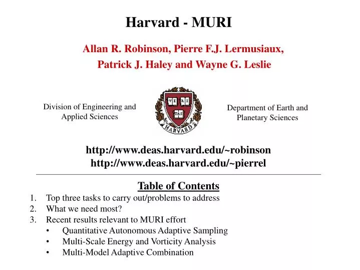
1. Harvard - MURI Allan R. Robinson, Pierre F.J. Lermusiaux, Patrick J. Haley and Wayne G. Leslie Division of Engineering and Applied Sciences Department of Earth and Planetary Sciences http://www.deas.harvard.edu/~robinson http://www.deas.harvard.edu/~pierrel • Table of Contents • Top three tasks to carry out/problems to address • What we need most? • Recent results relevant to MURI effort • Quantitative Autonomous Adaptive Sampling • Multi-Scale Energy and Vorticity Analysis • Multi-Model Adaptive Combination

2. Top Three Tasks to Carry Out/Problems to Address • Determine details of three metrics for adaptive sampling (coverage, dynamics, uncertainties) and develop schemes and exercise software for their integrated use • Carry out cooperative real-time data-driven predictions with adaptive sampling • Advance scientific understanding of 3D upwelling/relaxation dynamics and carry out budget analyses as possible

3. What Do We Need Most? • Effective collaboration • Integrated software • Good quality data with error estimates

4. Determine details of three metrics for adaptive sampling and develop schemes and exercise software for their integrated use • The three metrics: • Coverage (maintain synoptic accuracy) • Dynamics (maximize sampling of predicted dynamical events) • Uncertainty (minimize predicted uncertainties) • Integrate these adaptive sampling metrics and schemes with platform control and LCS metrics and schemes • Multiple platforms of different types used together in overall conceptual framework • Adaptive sampling schemes and software in pre-exercise simulations • Continue development of ESSE and MsEVA nonlinear adaptive sampling • Implement simple glider/AUV models within HOPS for i) measurement model and ii) data predictions • Continue development error models for HOPS and for glider/AUV/ship/aircraft data (with experimentalists)

5. Carry-out real-time data-driven predictions with adaptive sampling • Work in real-time with a committed general team of experimentalists and carry out adaptive sampling • Link and/or integrate HOPS with control theory and LCS software • Carry out real-time HOPS/ESSE (sub)-mesoscale field and uncertainty predictions with integrated 3-metrics adaptive sampling • 1-way and/or 2-way nested HOPS simulations (333m into 1km into 3km) • Sub-mesoscale effects including tidal effects • Efficient measures and assessment of predictive skill • Real-time forecast skill and hindcast skill of fields and uncertainties • Theory and software to measure skill of upwelling center/plume estimate: e.g. shape/size of plume, scales of jet and eddies at plume edges, thickness of boundary layers, surface/bottom fluxes • Real-time physical-acoustical DA with MIT and real-time biological-physical DA as possible with collaborators

6. Advance scientific understanding of 3D upwelling/relaxation dynamics and carry-out budget analyses on several scales • Develop and implement software for momentum, heat and mass budgets • On several scales and term-balances: e.g. point-by-point, time-dependent plume-averaged, Ms-EVA, etc. • Compare data-based budgets to data-model-based budgets • Science-focused studies of sensitivity of upwelling/relaxation processes • e.g. effects of atmospheric conditions and resolution, idealized geometries, tides/internal tides or boundary layer formulations on plume formation and relaxation • Improve model parameterizations based on model-data misfits (local and budgets) • Estimate predictability limits for upwelling/relaxation processes

7. What Do We Need Most? • Effective collaboration, rapid and efficient communication and real integrated system and system software • Effective integration of software • LCS with HOPS • Glider/AUV models with HOPS • Good forcing functions and good initial conditions • Real-time inter-calibration data stations to avoid false circulation features • Occasional and simultaneous sampling by pairs of platforms, efficiently scheduled by real-time control groups • Documented feedback from experimentalists • Both in real-time and after experiment

8. Quantitative Adaptive Sampling via ESSE • Select sets of candidate sampling paths/regions and variables that satisfy operational constraints • Forecast reduction of errors for each set based on a tree structure of small ensembles and data assimilation • Optimization of sampling plan: select sequence of paths/regions and sensor variables which maximize the predicted nonlinear error reduction in the spatial domain of interest, either at tf(trace of ``information matrix’’ at final time) or over [t0 , tf ] • Outputs: • Maps of predicted error reduction for each sampling paths/regions • Information (summary) maps: assigns to the location of each sampling region/path the average error reduction over domain of interest • Ideal sequence of paths/regions and variables to sample

9. ESSE fcts after DA of each track IC(nowcast) Forecast DA ESSE for Track 1 DA 1 ESSE for Track 2 DA 2 2-day ESSE fct ESSE for Track 3 DA 3 ESSE for Track 4 DA 4 Aug 24 Aug 27 Aug 26 Which sampling on Aug 26 optimally reduces uncertainties on Aug 27? 4 candidate tracks, overlaid on surface T fct for Aug 26

10. tracki 1. Define relative error reduction as: (27 - 27 ) / 27…..for 27 > noise 0………………for 27  noise 2. Create relative error reduction maps for each sampling tracks, e.g.: Which sampling on Aug 26 optimally reduces uncertainties on Aug 27? • Compute average over domain of interest for each variable, e.g. for full domain: Best to worst error reduction: Track 1 (18%), Pt Lobos (17%), …., Track 3 (6%) • Create “Aug 26 information map”: indicates where to sample on Aug 26 for optimal error reduction on Aug 27

11. Multi-Scale Energy and Vorticity Analysis August 19 August 20 August 18 August 19 August 18 August 20 August 21 August 22 August 23 August 21 August 22 August 23 • Multiscale window decomposition in space and time (wavelet-based) of energy/vorticity eqns. • For example, consider Energetics During Relaxation Period: Large-scale Kinetic Energy (KE) Large-scale Available Potential Energy (APE) • Both APE and KE decrease during the relaxation period • Transfer from large-scale window to mesoscale window occurs to account for decrease in large-scale energies (as confirmed by transfer and mesoscale terms) Windows: Large-scale (>= 8days; > 30km), mesoscale (0.5-8 days), and sub-mesoscale (< 0.5 days) Dr. X. San Liang

12. Approaches to Multi-Model Adaptive Forecasting Combine ROMS/HOPS re-analysis temperatures to fit the M2-buoy temperature at 10 m • By combining the models x1 and x2 we attempt to: • eliminate and learn systematic errors • reduce random errors • Approach utilized here: neural networks • A neural network is a non-linear operator which can be adapted (trained) to approximate a target arbitrary non-linear function measuring model-data misfits: Sigmoidal Transfer Function d Two fits tested i) Linear least-squares: ii) Single Sigmoidal layer: Oleg Logoutov

13. Neural Network Least Squares Fit Linear Least Squares Fit Equal Weights Individual Models • Observed (black) temp at the M2mooring • Modeled temp at the M2mooring: • ROMS re-analysis, HOPS re-analysis Top: Green – HOPS/ROMS reanalysis combined via neural network trained on the first subset of data (before Aug 17). Bottom: Green – HOPS/ROMS reanalysis combined via adaptive neural network also trained on the first subset of data (before Aug 17), but over moving-window of 3 days decorrelation

14. Extra Vugrafs

15. Aug 12 Aug 13 Aug 14 Start of Upwelling First Upwelling period End of Relaxation Second Upwelling period ESSE Surface Temperature Error Standard Deviation Forecasts Aug 27 Aug 24 Aug 28

16. ESSE: Uncertainty Predictions and Data Assimilation • Dynamics: dx =M(x)dt+ d~ N(0, Q) • Measurement: y = H(x) +  ~ N(0, R) • Non-lin. Err. Cov. evolution: • Error reduction by DA: P(0)=P0 where K is the reduced Kalman Gain • ESSE retains and nonlinearly evolves uncertainties that matter,combining, • Proper Orthogonal Decompositions (PODs) orKarhunen-Loeve (KL) expansions • Time-varying basis functions, and, • Multi-scale initialisation and Stochastic ensemble predictions • to obtain a dynamic low-dimensional representation of the error space. • Linked to Polynomial chaos, but • with time-varying error KL basis:

17. Adaptive sampling schemes via ESSE Adaptive Sampling: Use forecasts and their uncertainties to predict the most useful observation system in space (locations/paths) and time (frequencies) Dynamics: dx =M(x)dt+ d~ N(0, Q) Measurement: y = H(x) +  ~ N(0, R) Non-lin. Err. Cov.: Adaptive Sampling Metric or Cost function: e.g. Find Hi and Ri such that

18. Modeling of tidal effects in HOPS • Obtain first estimate of principal tidal constituents via a shallow water model • Global TPXO5 fields (Egbert, Bennett et al.) • Nested regional OTIS inversion using tidal-gauges and TPX05 at open-boundary • Used to estimate hierarchy of tidal parameterizations : • Vertical tidal Reynolds stresses (diff., visc.)KT =  ||uT||2and K=max(KS, KT) • Modification of bottom stress =CD ||uS+ uT ||uS • Horiz. momentum tidal Reyn. stresses (Reyn. stresses averaged over own T) • Horiz. tidal advection of tracers ½ free surface • Forcing for free-surface HOPS full free surface

19. T section across Monterey-Bay Temp. at 10 m Two 6-day model runs No-tides • Tidal effects • Vert. Reyn. Stress • Horiz. Momentum Stress

20. Post-Cruise Surface CHL forecast (Hindcast) • Starts from zeroth-order dynamically balanced IC on Aug 4 • Then, 13 days of physical DA • Forecast of 3-5 days afterwards CHL Aug 20 CHL Aug 21 CHL Aug 20, 20:00 GMT CHL Aug 22