Download

1 / 50
500 likes | 757 Views
Relative Valuation. What is relative valuation?. In relative valuation, the value of an asset is compared to the values assessed by the market for similar or comparable assets. To do relative valuation then, we need to identify comparable assets and obtain market values for these assets

E N D
What is relative valuation? • In relative valuation, the value of an asset is compared to the values assessed by the market for similar or comparable assets. • To do relative valuation then, • we need to identify comparable assets and obtain market values for these assets • convert these market values into standardized values, since the absolute prices cannot be compared This process of standardizing creates price multiples. • compare the standardized value or multiple for the asset being analyzed to the standardized values for comparable asset, controlling for any differences between the firms that might affect the multiple, to judge whether the asset is under or over valued
Relative valuation is pervasive… • Most valuations on Wall Street are relative valuations. • Almost 85% of equity research reports are based upon a multiple and comparables. • More than 50% of all acquisition valuations are based upon multiples • Rules of thumb based on multiples are not only common but are often the basis for final valuation judgments. • While there are more discounted cashflow valuations in consulting and corporate finance, they are often relative valuations masquerading as discounted cash flow valuations. • The objective in many discounted cashflow valuations is to back into a number that has been obtained by using a multiple. • The terminal value in a significant number of discounted cashflow valuations is estimated using a multiple.
The Market Imperative…. • Relative valuation is much more likely to reflect market perceptions and moods than discounted cash flow valuation. This can be an advantage when it is important that the price reflect these perceptions as is the case when • the objective is to sell a security at that price today (as in the case of an IPO) • investing on “momentum” based strategies • With relative valuation, there will always be a significant proportion of securities that are under valued and over valued. • Since portfolio managers are judged based upon how they perform on a relative basis (to the market and other money managers), relative valuation is more tailored to their needs • Relative valuation generally requires less information than discounted cash flow valuation (especially when multiples are used as screens)
Why relative valuation? “If you think I’m crazy, you should see the guy who lives across the hall” Jerry Seinfeld talking about Kramer in a Seinfeld episode “ A little inaccuracy sometimes saves tons of explanation” H.H. Munro “ If you are going to screw up, make sure that you have lots of company” Ex-portfolio manager
So, you believe only in intrinsic value? Here is why you should still care about relative value • Even if you are a true believer in discounted cashflow valuation, presenting your findings on a relative valuation basis will make it more likely that your findings/recommendations will reach a receptive audience. • In some cases, relative valuation can help find weak spots in discounted cash flow valuations and fix them. • The problem with multiples is not in their use but in their abuse. If we can find ways to frame multiples right, we should be able to use them better.
Standardizing Value • You can standardize either the equity value of an asset or the value of the asset itself, which goes in the numerator. • You can standardize by dividing by the • Earnings of the asset • Price/Earnings Ratio (PE) and variants (PEG and Relative PE) • Value/EBIT • Value/EBITDA • Value/Cash Flow • Book value of the asset • Price/Book Value(of Equity) (PBV) • Value/ Book Value of Assets • Value/Replacement Cost (Tobin’s Q) • Revenues generated by the asset • Price/Sales per Share (PS) • Value/Sales • Asset or Industry Specific Variable (Price/kwh, Price per ton of steel ....)
The Four Steps to Understanding Multiples • Define the multiple • In use, the same multiple can be defined in different ways by different users. When comparing and using multiples, estimated by someone else, it is critical that we understand how the multiples have been estimated • Describe the multiple • Too many people who use a multiple have no idea what its cross sectional distribution is. If you do not know what the cross sectional distribution of a multiple is, it is difficult to look at a number and pass judgment on whether it is too high or low. • Analyze the multiple • It is critical that we understand the fundamentals that drive each multiple, and the nature of the relationship between the multiple and each variable. • Apply the multiple • Defining the comparable universe and controlling for differences is far more difficult in practice than it is in theory.
Definitional Tests • Is the multiple consistently defined? • Proposition 1: Both the value (the numerator) and the standardizing variable ( the denominator) should be to the same claimholders in the firm. In other words, the value of equity should be divided by equity earnings or equity book value, and firm value should be divided by firm earnings or book value. • Is the multiple uniformly estimated? • The variables used in defining the multiple should be estimated uniformly across assets in the “comparable firm” list. • If earnings-based multiples are used, the accounting rules to measure earnings should be applied consistently across assets. The same rule applies with book-value based multiples.
Descriptive Tests • What is the average and standard deviation for this multiple, across the universe (market)? • What is the median for this multiple? • The median for this multiple is often a more reliable comparison point. • How large are the outliers to the distribution, and how do we deal with the outliers? • Throwing out the outliers may seem like an obvious solution, but if the outliers all lie on one side of the distribution (they usually are large positive numbers), this can lead to a biased estimate. • Are there cases where the multiple cannot be estimated? Will ignoring these cases lead to a biased estimate of the multiple? • How has this multiple changed over time?
Analytical Tests • What are the fundamentals that determine and drive these multiples? • Proposition 2: Embedded in every multiple are all of the variables that drive every discounted cash flow valuation - growth, risk and cash flow patterns. • In fact, using a simple discounted cash flow model and basic algebra should yield the fundamentals that drive a multiple • How do changes in these fundamentals change the multiple? • The relationship between a fundamental (like growth) and a multiple (such as PE) is seldom linear. For example, if firm A has twice the growth rate of firm B, it will generally not trade at twice its PE ratio • Proposition 3: It is impossible to properly compare firms on a multiple, if we do not know the nature of the relationship between fundamentals and the multiple.
Application Tests • Given the firm that we are valuing, what is a “comparable” firm? • While traditional analysis is built on the premise that firms in the same sector are comparable firms, valuation theory would suggest that a comparable firm is one which is similar to the one being analyzed in terms of fundamentals. • Proposition 4: There is no reason why a firm cannot be compared with another firm in a very different business, if the two firms have the same risk, growth and cash flow characteristics. • Given the comparable firms, how do we adjust for differences across firms on the fundamentals? • Proposition 5: It is impossible to find an exactly identical firm to the one you are valuing.
Price Earnings Ratio: Definition PE = Market Price per Share / Earnings per Share • There are a number of variants on the basic PE ratio in use. They are based upon how the price and the earnings are defined. • Price: is usually the current price is sometimes the average price for the year • EPS: earnings per share in most recent financial year earnings per share in trailing 12 months (Trailing PE) forecasted earnings per share next year (Forward PE) forecasted earnings per share in future year
Comparing PE Ratios: US, Europe, Japan and Emerging Markets - January 2005 Median PE Japan = 23.45 US = 23.21 Europe = 18.79 Em. Mkts = 16.18
PE Ratio: Understanding the Fundamentals • To understand the fundamentals, start with a basic equity discounted cash flow model. • With the dividend discount model, • Dividing both sides by the earnings per share, • If this had been a FCFE Model,
PE Ratio and Fundamentals • Proposition: Other things held equal, higher growth firms will have higher PE ratios than lower growth firms. • Proposition: Other things held equal, higher risk firms will have lower PE ratios than lower risk firms • Proposition: Other things held equal, firms with lower reinvestment needs will have higher PE ratios than firms with higher reinvestment rates. • Of course, other things are difficult to hold equal since high growth firms, tend to have risk and high reinvestment rats.
Using the Fundamental Model to Estimate PE For a High Growth Firm • The price-earnings ratio for a high growth firm can also be related to fundamentals. In the special case of the two-stage dividend discount model, this relationship can be made explicit fairly simply: • For a firm that does not pay what it can afford to in dividends, substitute FCFE/Earnings for the payout ratio. • Dividing both sides by the earnings per share:
Expanding the Model • In this model, the PE ratio for a high growth firm is a function of growth, risk and payout, exactly the same variables that it was a function of for the stable growth firm. • The only difference is that these inputs have to be estimated for two phases - the high growth phase and the stable growth phase. • Expanding to more than two phases, say the three stage model, will mean that risk, growth and cash flow patterns in each stage.
A Simple Example • Assume that you have been asked to estimate the PE ratio for a firm which has the following characteristics: Variable High Growth Phase Stable Growth Phase Expected Growth Rate 25% 8% Payout Ratio 20% 50% Beta 1.00 1.00 Number of years 5 years Forever after year 5 • Riskfree rate = T.Bond Rate = 6% • Required rate of return = 6% + 1(5.5%)= 11.5%
PE, Growth and Risk Dependent variable is: PE R squared = 66.2% R squared (adjusted) = 63.1% Variable Coefficient SE t-ratio prob Constant 13.1151 3.471 3.78 0.0010 Growth rate 121.223 19.27 6.29 ≤ 0.0001 Emerging Market -13.8531 3.606 -3.84 0.0009 Emerging Market is a dummy: 1 if emerging market 0 if not
Is Telebras under valued? • Predicted PE = 13.12 + 121.22 (.075) - 13.85 (1) = 8.35 • At an actual price to earnings ratio of 8.9, Telebras is slightly overvalued. • Given the R-squared on the regression, though, a more precise statistical statement would be that the predicated PE for Telebras will fall within a range. In this case, the range would be as follows: • Upper end of the range: 10.06 • Lower end of the range: 6.64 • As a general rule, the higher the R-squared the narrower the range for the predicted values. The range will also tend to be tighter for firms that fall close to the average and become wider for extreme values.
Using the entire crosssection: A regression approach • In contrast to the 'comparable firm' approach, the information in the entire cross-section of firms can be used to predict PE ratios. • The simplest way of summarizing this information is with a multiple regression, with the PE ratio as the dependent variable, and proxies for risk, growth and payout forming the independent variables.
Problems with the regression methodology • The basic regression assumes a linear relationship between PE ratios and the financial proxies, and that might not be appropriate. • The basic relationship between PE ratios and financial variables itself might not be stable, and if it shifts from year to year, the predictions from the model may not be reliable. • The independent variables are correlated with each other. For example, high growth firms tend to have high risk. This multi-collinearity makes the coefficients of the regressions unreliable and may explain the large changes in these coefficients from period to period.
Value/Earnings and Value/Cashflow Ratios • While Price earnings ratios look at the market value of equity relative to earnings to equity investors, Value earnings ratios look at the market value of the firm relative to operating earnings. Value to cash flow ratios modify the earnings number to make it a cash flow number. • The form of value to cash flow ratios that has the closest parallels in DCF valuation is the value to Free Cash Flow to the Firm, which is defined as: Value/FCFF = (Market Value of Equity + Market Value of Debt-Cash) EBIT (1-t) - (Cap Ex - Deprecn) - Chg in WC • Consistency Tests: • If the numerator is net of cash (or if net debt is used, then the interest income from the cash should not be in denominator • The interest expenses added back to get to EBIT should correspond to the debt in the numerator. If only long term debt is considered, only long term interest should be added back.
Value of Firm/FCFF: Determinants • Reverting back to a two-stage FCFF DCF model, we get: • V0 = Value of the firm (today) • FCFF0 = Free Cashflow to the firm in current year • g = Expected growth rate in FCFF in extraordinary growth period (first n years) • WACC = Weighted average cost of capital • gn = Expected growth rate in FCFF in stable growth period (after n years)
Value Multiples • Dividing both sides by the FCFF yields, • The value/FCFF multiples is a function of • the cost of capital • the expected growth
Reasons for Increased Use of Value/EBITDA 1. The multiple can be computed even for firms that are reporting net losses, since earnings before interest, taxes and depreciation are usually positive. 2. For firms in certain industries, such as cellular, which require a substantial investment in infrastructure and long gestation periods, this multiple seems to be more appropriate than the price/earnings ratio. 3. In leveraged buyouts, where the key factor is cash generated by the firm prior to all discretionary expenditures, the EBITDA is the measure of cash flows from operations that can be used to support debt payment at least in the short term. 4. By looking at cashflows prior to capital expenditures, it may provide a better estimate of “optimal value”, especially if the capital expenditures are unwise or earn substandard returns. 5. By looking at the value of the firm and cashflows to the firm it allows for comparisons across firms with different financial leverage.
Value/EBITDA Multiple • The Classic Definition • The No-Cash Version • When cash and marketable securities are netted out of value, none of the income from the cash and securities should be reflected in the denominator.
The Determinants of Value/EBITDA Multiples: Linkage to DCF Valuation • Firm value can be written as: • The numerator can be written as follows: FCFF = EBIT (1-t) - (Cex - Depr) - Working Capital = (EBITDA - Depr) (1-t) - (Cex - Depr) - Working Capital = EBITDA (1-t) + Depr (t) - Cex - Working Capital
From Firm Value to EBITDA Multiples • Now the Value of the firm can be rewritten as, • Dividing both sides of the equation by EBITDA,
A Simple Example • Consider a firm with the following characteristics: • Tax Rate = 36% • Capital Expenditures/EBITDA = 30% • Depreciation/EBITDA = 20% • Cost of Capital = 10% • The firm has no working capital requirements • The firm is in stable growth and is expected to grow 5% a year forever.
Calculating Value/EBITDA Multiple • In this case, the Value/EBITDA multiple for this firm can be estimated as follows:
Price Sales Ratio: Definition • The price/sales ratio is the ratio of the market value of equity to the sales. • Price/ Sales= Market Value of Equity Total Revenues • Consistency Tests • The price/sales ratio is internally inconsistent, since the market value of equity is divided by the total revenues of the firm.
Price/Sales Ratio: Determinants • The price/sales ratio of a stable growth firm can be estimated beginning with a 2-stage equity valuation model: • Dividing both sides by the sales per share:
Choosing Between the Multiples • As presented in this section, there are dozens of multiples that can be potentially used to value an individual firm. • In addition, relative valuation can be relative to a sector (or comparable firms) or to the entire market (using the regressions, for instance) • Since there can be only one final estimate of value, there are three choices at this stage: • Use a simple average of the valuations obtained using a number of different multiples • Use a weighted average of the valuations obtained using a nmber of different multiples • Choose one of the multiples and base your valuation on that multiple
Picking one Multiple • This is usually the best way to approach this issue. While a range of values can be obtained from a number of multiples, the “best estimate” value is obtained using one multiple. • The multiple that is used can be chosen in one of two ways: • Use the multiple that best fits your objective. Thus, if you want the company to be undervalued, you pick the multiple that yields the highest value. • Use the multiple that has the highest R-squared in the sector when regressed against fundamentals. Thus, if you have tried PE, PBV, PS, etc. and run regressions of these multiples against fundamentals, use the multiple that works best at explaining differences across firms in that sector. • Use the multiple that seems to make the most sense for that sector, given how value is measured and created.
A More Intuitive Approach • Managers in every sector tend to focus on specific variables when analyzing strategy and performance. The multiple used will generally reflect this focus. Consider three examples. • In retailing: The focus is usually on same store sales (turnover) and profit margins. Not surprisingly, the revenue multiple is most common in this sector. • In financial services: The emphasis is usually on return on equity. Book Equity is often viewed as a scarce resource, since capital ratios are based upon it. Price to book ratios dominate. • In technology: Growth is usually the dominant theme. PEG ratios were invented in this sector.
In Practice… • As a general rule of thumb, the following table provides a way of picking a multiple for a sector Sector Multiple Used Rationale Cyclical Manufacturing PE, Relative PE Often with normalized earnings High Tech, High Growth PEG Big differences in growth across firms High Growth/No Earnings PS, VS Assume future margins will be good Heavy Infrastructure VEBITDA Firms in sector have losses in early years and reported earnings can vary depending on depreciation method REITa P/CF Generally no cap ex investments from equity earnings Financial Services PBV Book value often marked to market Retailing PS If leverage is similar across firms VS If leverage is different
Reviewing: The Four Steps to Understanding Multiples • Define the multiple • Check for consistency • Make sure that they are estimated uniformly • Describe the multiple • Multiples have skewed distributions: The averages are seldom good indicators of typical multiples • Check for bias, if the multiple cannot be estimated • Analyze the multiple • Identify the companion variable that drives the multiple • Examine the nature of the relationship • Apply the multiple