Download
1 / 80
800 likes | 996 Views
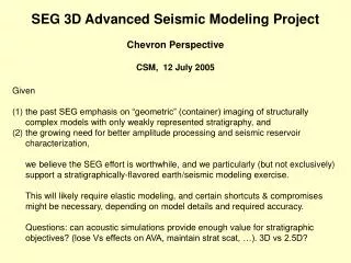
SEG 3D Advanced Seismic Modeling Project Chevron Perspective CSM, 12 July 2005 Houston(Hess), 8 Sept 2005 Houston(COP), 14 Oct 2005. Given the past SEG emphasis on “geometric” (container) imaging of structurally complex models with only weakly represented stratigraphy, and

E N D
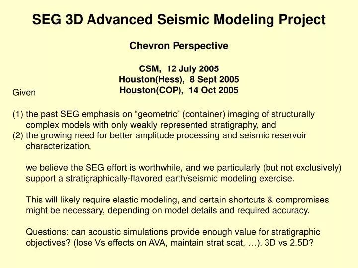
SEG 3D Advanced Seismic Modeling Project Chevron Perspective CSM, 12 July 2005 Houston(Hess), 8 Sept 2005 Houston(COP), 14 Oct 2005 • Given • the past SEG emphasis on “geometric” (container) imaging of structurally complex models with only weakly represented stratigraphy, and • the growing need for better amplitude processing and seismic reservoir characterization, • we believe the SEG effort is worthwhile, and we particularly (but not exclusively) support a stratigraphically-flavored earth/seismic modeling exercise. • This will likely require elastic modeling, and certain shortcuts & compromises might be necessary, depending on model details and required accuracy. • Questions: can acoustic simulations provide enough value for stratigraphic objectives? (lose Vs effects on AVA, maintain strat scat, …). 3D vs 2.5D?
A Recipe for Realistic Stratigraphy Construction SEG 3D Advanced Seismic Modeling Project Joe Stefani, Chevron CSM, 12 July 2005 Houston, 8 Sept 2005
Towards Realistic Seismic Earth Models: • Evolution of Earth/Strat Models • 1 Matching key property and correlation characteristics • 2 Generating flat stratigraphy • 3 Adding interesting reservoirs in 3D • 4 Warping/Morphing by hand • 4 Warping/Morphing by inverse flattening • 5 Applying mild near-surface velocity perturbations • 6 Masking-in a salt body (for structural problem)
1: Match Key Property and Correlation Characteristics Want the model to match the Earth in these (necessary but maybe insufficient) characteristics: spatial correlation of property variations horizontally and vertically RMS of property fluctuations about local mean histogram of property fluctuations about local mean correlation coefficients among Vp,Vs,Dn reflectivities Background on Spatial Correlation of Property Variations: Statistical Self-Similarity and Power Laws
Illustration of Self-Affinity: Vertical Vp Log at 3 scales (depth in feet, linear trend removed, power = 1.2: horzfac=2 vertfac=2b/2 =1.5) Depth (ft)
Seismic Parameters for strat5 Model (VE=3) Vp 2Vs 4000Den
Vp 2Vs 4000Den Reflectivity*Wavelet Depth Sections VE=5 Time Section
Alternative Slope Valley AnalogueNigeria, Deptuc et al. 2003
Channels with Levies and Downslope-Migrating Loops Plan view of a vertical average of Vshale: (white=0, red=1) 5 km Direction of flow 10 km Cellular resolution: dx = dy = 25m, dz = 4m
Cross-Section of Channels with Levies Model Vshale: (white=0, red=1) Vert Exag = 10:1 200 m 5 km
Multi Layer Interpretation Distributary channel interpretation from 14 time slices thoughout 12.5 interval, merged to show channel stacking & switching pattern
Anastomosing & Constricted Channels without Levies (spaghetti model) Plan view of a vertical average of Vshale: (white=0, red=1) 5 km 10 km Cellular resolution: dx = dy = 25m, dz = 4m
Cross-Section (near throat) of Spaghetti Model Vshale: (white=0, red=1) Vert Exag = 20:1 100 m 5 km
Strat example 2: Braided channels + overbank meander channel
‘Transient Fan’ West Channel Channels (Bypass Facies) Channels (Channel fill Facies) East Channel ‘Transient Fans’ Depositional Lobes (Stacked Sheet Facies) ‘Terminal Fan’ MUD DIAPIR 2500m Transient FansShallow Seismic Examples from Nigeria Dayo Adeogbas (2003)
3D Conceptual Models Water depth = 1000m Overburden = 2000m 10km 2km 100m 3000-5000m Stratigraphic cell resolution = 25m x 25m x 1m Seismic cell resolution = 25m x 25m x5m
Jurassic Tank 3D VolumeUniversity of Minnesota, St. Anthony Falls Laboratorycourtesy of Prof. Chris Paola
Dip Section B B’ Stratigraphers call this ~alluvial fan delta, and suggest vertical scale should be 0.2 to 0.5 of what is shown at left. This sand-rich system contains 63% sand (blue), 27% coal (non-blue) and 10% kaolinite. Also, vertical exaggeration is estimated ~5:1
Dip Section B B’
A’ A Strike Section
Strike Section ~30 meters (<50m) Stratigraphers would call this ~alluvial fan delta, and would scale it vertically according to bar at right, with VE ~ 5:1
Water well control Top Res Bot Res Reservoir embedded in stratigraphic container for seismic modeling
Depth slice through reservoir Realistic stratigraphic earth models provide a good testbed for various stochastic spatial inversion methods used in reservoir modeling and flow prediction. fault
2D Stratigraphic Earth Model 2D Elastic Finite Difference, prestack time migration, stack
Seismic – med freq (1D convolution) Kuito interval
Flattening overviewJesse Lomask, Antoine Guitton, Sergey Fomel, Jon Claerbout, and Alejandro ValencianoStanford Exploration Project Estimate local dip fieldSum the dipsApply summed dips as time shifts
Measure 2D dip vector & Estimate 3D t field General idea:
Depth (m) CMP Downlap picks Iteration: 0
Depth (m) CMP Downlap picks Iteration: 10
900 4000 8000 13000 4500 Y (m) 3800 Depth (m) X (m)
900 4000 8000 13000 200 x 300 x 60 ~20 minutes 4500 Y (m) 3800 Depth (m) X (m)
Inverse flattening begins with flat synthetic strat and warps it according to red t field 900 Depth (m) 4000 X (m) 8000 13000