Download
1 / 40
400 likes | 512 Views
LBSC 796/INFM 718R: Week 4 Language Models. Jimmy Lin College of Information Studies University of Maryland Monday, February 20, 2006. Last Time…. Boolean model Based on the notion of sets Documents are retrieved only if they satisfy Boolean conditions specified in the query

E N D
LBSC 796/INFM 718R: Week 4Language Models Jimmy Lin College of Information Studies University of Maryland Monday, February 20, 2006
Last Time… • Boolean model • Based on the notion of sets • Documents are retrieved only if they satisfy Boolean conditions specified in the query • Does not impose a ranking on retrieved documents • Exact match • Vector space model • Based on geometry, the notion of vectors in high dimensional space • Documents are ranked based on their similarity to the query (ranked retrieval) • Best/partial match
Today • Language models • Based on the notion of probabilities and processes for generating text • Documents are ranked based on the probability that they generated the query • Best/partial match • First we start with probabilities…
Probability • What is probability? • Statistical: relative frequency as n • Subjective: degree of belief • Thinking probabilistically • Imagine a finite amount of “stuff” (= probability mass) • The total amount of “stuff” is one • The event space is “all the things that could happen” • Distribute that “mass” over the possible events • Sum of all probabilities have to add up to one
Key Concepts • Defining probability with frequency • Statistical independence • Conditional probability • Bayes’ Theorem
Statistical Independence • A and B are independent if and only if: • P(A and B) = P(A) P(B) • Simplest example: series of coin flips • Independence formalizes “unrelated” • P(“being brown eyed”) = 6/10 • P(“being a doctor”) = 1/1000 • P(“being a brown eyed doctor”) = P(“being brown eyed”) P(“being a doctor”) = 6/10,000
Dependent Events • Suppose: • P(“having a B.S. degree”) = 4/10 • P(“being a doctor”) = 1/1000 • Would you expect: • P(“having a B.S. degree and being a doctor”) = P(“having a B.S. degree”) P(“being a doctor”)= 4/10,000 • Another example: • P(“being a doctor”) = 1/1000 • P(“having studied anatomy”) = 12/1000 • P(“having studied anatomy” | “being a doctor”) = ??
Conditional Probability P(A | B) P(A and B) / P(B) Event Space A and B A B P(A) = prob. of A relative to entire event space P(A|B) = prob. of A considering that we know B is true
Doctors and Anatomy P(A | B) P(A and B) / P(B) What is P(“having studied anatomy” | “being a doctor”)? A = having studied anatomy B = being a doctor P(“being a doctor”) = 1/1000 P(“having studied anatomy”) = 12/1000 P(“being a doctor who studied anatomy”) = 1/1000 P(“having studied anatomy” | “being a doctor”) = 1
More on Conditional Probability • What if P(A|B) = P(A)? • Is P(A|B) = P(B|A)? A and B must be statistically independent! A = having studied anatomy B = being a doctor P(“being a doctor”) = 1/1000 P(“having studied anatomy”) = 12/1000 P(“being a doctor who studied anatomy”) = 1/1000 P(“having studied anatomy” | “being a doctor”) = 1 If you’re a doctor, you must have studied anatomy… P(“being a doctor” | “having studied anatomy”) = 1/12 If you’ve studied anatomy, you’re more likely to be a doctor, but you could also be a biologist, for example
Probabilistic Inference • Suppose there’s a horrible, but very rare disease • But there’s a very accurate test for it • Unfortunately, you tested positive… The probability that you contracted it is 0.01% The test is 99% accurate Should you panic?
Prior probability Posterior probability Bayes’ Theorem • You want to find • But you only know • How rare the disease is • How accurate the test is • Use Bayes’ Theorem (hence Bayesian Inference) P(“have disease” | “test positive”)
Applying Bayes’ Theorem • P(“have disease”) = 0.0001 (0.01%) • P(“test positive” | “have disease”) = 0.99 (99%) • P(“test positive”) = 0.010098 • Two case: • You have the disease, and you tested positive • You don’t have the disease, but you tested positive (error) Case 1: (0.0001)(0.99) = 0.000099 Case 2: (0.9999)(0.01) = 0.009999 Case 1+2 = 0.010098 P(“have disease” | “test positive”) = (0.99)(0.0001) / 0.010098 = 0.009804 = 0.9804% Don’t worry!
Another View In a population of one million people 100 are infected 999,900 are not 99 test positive 1 test negative 9999 test positive 989901 test negative 10098 will test positive… Of those, only 99 really have the disease!
Competing Hypotheses • Consider • A set of hypotheses: H1, H2, H3 • Some observable evidence: O • If you observed O, what likely caused it? • Example: • You know that three things can cause the grass to be wet: rain, sprinkler, flood • You observed that that grass is wet • What caused it? P1 = P(H1|O) P2 = P(H2|O) P3 = P(H3|O) Which explanation is most likely?
An Example • Let • O = “Joe earns more than $80,000/year” • H1 = “Joe is a NBA referee” • H2 = “Joe is a college professor” • H3 = “Joe works in food services” • Suppose we know that Joe earns more than $80,000 a year… • What should be our guess about Joe’s profession?
What’s his job? • Suppose we do a survey and we find out • P(O|H1) = 0.6 P(H1) = 0.0001 referee • P(O|H2) = 0.07 P(H2) = 0.001 professor • P(O|H3) = 0.001 P(H3) = 0.02 food services • We can calculate • P(H1|O) = 0.00006 / P(“earning > $80K/year”) • P(H2|O) = 0.00007 / P(“earning > $80K/year”) • P(H3|O) = 0.00002 / P(“earning > $80K/year”) • What do we guess?
Recap: Key Concepts • Defining probability with frequency • Statistical independence • Conditional probability • Bayes’ Theorem
What is a Language Model? • Probability distribution over strings of text • How likely is a string in a given “language”? • Probabilities depend on what language we’re modeling p1 = P(“a quick brown dog”) p2 = P(“dog quick a brown”) p3 = P(“быстрая brown dog”) p4 = P(“быстраясобака”) In a language model for English: p1 > p2 > p3 > p4 In a language model for Russian: p1 < p2 < p3 < p4
How do we model a language? • Brute force counts? • Think of all the things that have ever been said or will ever be said, of any length • Count how often each one occurs • Is understanding the path to enlightenment? • Figure out how meaning and thoughts are expressed • Build a model based on this • Throw up our hands and admit defeat?
Unigram Language Model • Assume each word is generated independently • Obviously, this is not true… • But it seems to work well in practice! • The probability of a string, given a model: The probability of a sequence of words decomposes into a product of the probabilities of individual words
P ( ) P ( ) P ( ) P ( ) P ( ) = A Physical Metaphor • Colored balls are randomly drawn from an urn (with replacement) M words = (4/9) (2/9) (4/9) (3/9)
Model M P(w) w 0.2 the 0.1 a 0.01 man 0.01 woman 0.03 said 0.02 likes … An Example the man likes the woman 0.2 0.01 0.02 0.2 0.01 multiply P(s | M) = 0.00000008 P(“the man likes the woman”|M) = P(the|M) P(man|M) P(likes|M) P(the|M) P(man|M) = 0.00000008
the class pleaseth yon maiden 0.2 0.01 0.0001 0.0001 0.0005 0.2 0.001 0.02 0.1 0.01 Comparing Language Models Model M1 Model M2 P(w) w 0.2 the 0.0001 yon 0.01 class 0.0005 maiden 0.0003 sayst 0.0001 pleaseth … P(w) w 0.2 the 0.1 yon 0.001 class 0.01 maiden 0.03 sayst 0.02 pleaseth … P(s|M2) > P(s|M1) What exactly does this mean?
Noisy-Channel Model of IR Information need d1 d2 Query … User has a information need, “thinks” of a relevant document… and writes down some queries dn document collection Task of information retrieval: given the query, figure out which document it came from?
Transmitter Receiver Decoder How is this a noisy-channel? • No one seriously claims that this is actually what’s going on… • But this view is mathematically convenient! Source Destination message channel message noise Source Destination Information need query terms Encoder channel Query formulation process
Retrieval w/ Language Models • Build a model for every document • Rank document d based on P(MD | q) • Expand using Bayes’ Theorem • Same as ranking by P(q | MD) P(q) is same for all documents; doesn’t change ranks P(MD) [the prior] is assumed to be the same for all d
Hey, what’s the probability this query came from you? Hey, what’s the probability that you generated this query? model1 model1 Hey, what’s the probability this query came from you? Hey, what’s the probability that you generated this query? model2 model2 Hey, what’s the probability this query came from you? Hey, what’s the probability that you generated this query? modeln modeln What does it mean? Ranking by P(MD | q)… is the same as ranking by P(q | MD) … …
Hey, what’s the probability that you generated this query? model1 … is a model of document1 Hey, what’s the probability that you generated this query? … is a model of document2 model2 Hey, what’s the probability that you generated this query? … is a model of documentn modeln Ranking Models? Ranking by P(q | MD) … is the same as ranking documents …
Building Document Models • How do we build a language model for a document? What’s in the urn? Physical metaphor: M What colored balls and how many of each?
A First Try • Simply count the frequencies in the document = maximum likelihood estimate M Sequence S P ( ) = 1/2 P ( ) = 1/4 P ( ) = 1/4 P(w|MS) = #(w,S) / |S| #(w,S) = number of times w occurs in S |S| = length of S
M P ( ) = 1/2 P ( ) = 1/4 P ( ) = 1/4 P ( ) P ( ) P ( ) P ( ) = P ( ) Zero-Frequency Problem • Suppose some event is not in our observation S • Model will assign zero probability to that event Sequence S !! = (1/2) (1/4) 0 (1/4) = 0
Why is this a bad idea? • Modeling a document • Just because a word didn’t appear doesn’t mean it’ll never appear… • But safe to assume that unseen words are rare • Think of the document model as a topic • There are many documents that can be written about a single topic • We’re trying to figure out what the model is based on just one document • Practical effect: assigning zero probability to unseen words forces exact match • But partial matches are useful also! Analogy: fishes in the sea
Smoothing The solution: “smooth” the word probabilities P(w) Maximum Likelihood Estimate Smoothed probability distribution w
How do you smooth? • Assign some small probability to unseen events • But remember to take away “probability mass” from other events • Simplest example: for words you didn’t see, pretend you saw it once • Other more sophisticated methods: • Absolute discounting • Linear interpolation, Jelinek-Mercer • Dirichlet, Witten-Bell • Good-Turing • … • Lots of performance to be gotten out of smoothing!
Recap: LM for IR • Build language models for every document • Models can be viewed as “topics” • Models are “generative” • Smoothing is very important • Retrieval: • Estimate the probability of generating the query according to each model • Rank the documents according to these probabilities
Advantages of LMs • Novel way of looking at the problem of text retrieval • Conceptually simple and explanatory • Unfortunately, not realistic • Formal mathematical model • Satisfies math envy • Natural use of collection statistics, not heuristics
Comparison With Vector Space • Similar in some ways • Term weights are based on frequency • Terms treated as if they were independent (unigram language model) • Probabilities have the effect of length normalization • Different in others • Based on probability rather than similarity • Intuitions are probabilistic (processes for generating text) rather than geometric • Details of use of document length and term, document, and collection frequencies differ
What’s the point? • Language models formalize assumptions • Binary relevance • Document independence • Term independence • Uniform priors • All of which aren’t true! • Relevance isn’t binary • Documents are often not independent • Terms are clearly not independent • Some documents are inherently higher in quality • But it works!
One Minute Paper • What was the muddiest point in today’s class?