Download
1 / 83
830 likes | 999 Views
Chapter 11: Analyzing the Association Between Categorical Variables. Section 11.1: What is Independence and What is Association?. Learning Objectives. Comparing Percentages Independence vs. Dependence.

E N D
Chapter 11: Analyzing the Association Between Categorical Variables Section 11.1: What is Independence and What is Association?
Learning Objectives • Comparing Percentages • Independence vs. Dependence
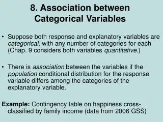
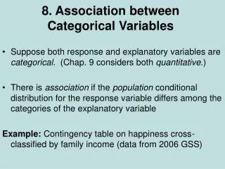
Learning Objective 1: Example: Is There an Association Between Happiness and Family Income?
Learning Objective 1: Example: Is There an Association Between Happiness and Family Income? • The percentages in a particular row of a table are calledconditional percentages • They form theconditional distributionfor happiness, given a particular income level
Learning Objective 1: Example: Is There an Association Between Happiness and Family Income?
Learning Objective 1: Example: Is There an Association Between Happiness and Family Income? • Guidelines when constructing tables with conditional distributions: • Make the response variable the column variable • Compute conditional proportions for the response variable within each row • Include the total sample sizes
Learning Objective 2:Independence vs. Dependence • For two variables to beindependent, the population percentage in any category of one variable is the same for all categories of the other variable • For two variables to bedependent (or associated),the population percentages in the categories are not all the same
Learning Objective 2:Independence vs. Dependence • Are race and belief in life after death independent or dependent? • The conditional distributions in the table are similar but not exactly identical • It is tempting to conclude that the variables are dependent
Learning Objective 2:Independence vs. Dependence • Are race and belief in life after death independent or dependent? • The definition of independence between variables refers to a population • The table is a sample, not a population
Learning Objective 2:Independence vs. Dependence • Even if variables are independent, we would not expect the sample conditional distributions to be identical • Because of sampling variability, eachsamplepercentage typically differs somewhat from thetrue populationpercentage
Chapter 11: Analyzing the Association Between Categorical Variables Section 11.2: How Can We Test Whether Categorical Variables Are Independent?
Learning Objectives • A Significance Test for Categorical Variables • What Do We Expect for Cell Counts if the Variables Are Independent? • How Do We Find the Expected Cell Counts? • The Chi-Squared Test Statistic • The Chi-Squared Distribution • The Five Steps of the Chi-Squared Test of Independence
Learning Objectives • Chi-Squared is Also Used as a “Test of Homogeneity” • Chi-Squared and the Test Comparing Proportions in 2x2 Tables • Limitations of the Chi-Squared Test
Learning Objective 1:A Significance Test for Categorical Variables • Create a table of frequencies divided into the categories of the two variables • The hypotheses for the test are: H0: The two variables are independent Ha: The two variables aredependent (associated) • The test assumes random sampling and a large sample size (cell counts in the frequency table of at least 5)
Learning Objective 2:What Do We Expect for Cell Counts if the Variables Are Independent? • The count in any particular cell is a random variable • Different samples have different countvalues • The mean of its distribution is called an expected cell count • This is found under the presumption that H0 is true
Learning Objective 3:How Do We Find the Expected Cell Counts? • Expected Cell Count: • For a particular cell, • The expected frequencies are values that have the same row and column totals as the observed counts, but for which the conditional distributions are identical (this is the assumption of the null hypothesis).
Learning Objective 3:How Do We Find the Expected Cell Counts?Example
Learning Objective 4:The Chi-Squared Test Statistic • The chi-squared statistic summarizes how far the observed cell counts in a contingency table fall from the expected cell counts for a null hypothesis
Learning Objective 4:Example: Happiness and Family Income • State the null and alternative hypotheses for this test • H0: Happiness and family income are independent • Ha: Happiness and family income are dependent (associated)
Learning Objective 4:Example: Happiness and Family Income • Report the statistic and explain how it was calculated: • To calculate the statistic, for each cell, calculate: • Sum the values for all the cells • The value is 73.4
Learning Objective 4:The Chi-Squared Test Statistic • The larger the value, the greater the evidence against the null hypothesis of independence and in support of the alternative hypothesis that happiness and income are associated
Learning Objective 5:The Chi-Squared Distribution • To convert the test statistic to a P-value, we use the sampling distribution of the statistic • For large sample sizes, this sampling distribution is well approximated by the chi-squared probability distribution
Learning Objective 5:The Chi-Squared Distribution • Main properties of the chi-squared distribution: • It falls on the positive part of the real number line • The precise shape of the distribution depends on the degrees of freedom: df = (r-1)(c-1)
Learning Objective 5:The Chi-Squared Distribution • Main properties of the chi-squared distribution: • The mean of the distribution equals the df value • It is skewed to the right • The larger the value, the greater the evidence against H0: independence
Learning Objective 6:The Five Steps of the Chi-Squared Test of Independence 1. Assumptions: • Two categorical variables • Randomization • Expected counts ≥ 5 in all cells
Learning Objective 6:The Five Steps of the Chi-Squared Test of Independence 2. Hypotheses: • H0: The two variables are independent • Ha: The two variables are dependent (associated)
Learning Objective 6:The Five Steps of the Chi-Squared Test of Independence 3.Test Statistic:
Learning Objective 6:The Five Steps of the Chi-Squared Test of Independence 4. P-value: Right-tail probability above the observedvalue, for the chi-squared distribution with df = (r-1)(c-1) 5. Conclusion: Report P-value and interpret in context • If a decision is needed, reject H0 when P-value ≤ significance level
Learning Objective 7:Chi-Squared is Also Used as a “Test of Homogeneity” • The chi-squared test does not depend on which is the response variable and which is the explanatory variable • When a response variable is identified and the population conditional distributions are identical, they are said to be homogeneous • The test is then referred to as a test of homogeneity
Learning Objective 8:Chi-Squared and the Test Comparing Proportions in 2x2 Tables • In practice, contingency tables of size 2x2 are very common. They often occur in summarizing the responses of two groups on a binary response variable. • Denote the population proportion of success by p1 in group 1 and p2 in group 2 • If the response variable is independent of the group, p1=p2, so the conditional distributions are equal • H0: p1=p2 is equivalent to H0: independence
Learning Objective 8:Example: Aspirin and Heart Attacks Revisited
Learning Objective 8: Example: Aspirin and Heart Attacks Revisited • What are the hypotheses for the chi-squared test for these data? • The null hypothesis is that whether a doctor has a heart attack is independent of whether he takes placebo or aspirin • The alternative hypothesis is that there’s an association
Learning Objective 8: Example: Aspirin and Heart Attacks Revisited • Report the test statistic and P-value for the chi-squared test: • The test statistic is 25.01 with a P-value of 0.000 • This is very strong evidence that the population proportion of heart attacks differed for those taking aspirin and for those taking placebo
Learning Objective 8: Example: Aspirin and Heart Attacks Revisited • The sample proportions indicate that the aspirin group had a lower rate of heart attacks than the placebo group
Learning Objective 9:Limitations of the Chi-Squared Test • If the P-value is very small, strong evidence exists against the null hypothesis of independence But… • The chi-squared statistic and the P-value tell us nothing about the nature of the strength of the association
Learning Objective 9:Limitations of the Chi-Squared Test • We know that there is statistical significance, but the test alone does not indicate whether there is practical significance as well
Learning Objective 9:Limitations of the Chi-Squared Test • The chi-squared test is often misused. Some examples are: • when some of the expected frequencies are too small • when separate rows or columns are dependent samples • data are not random • quantitative data are classified into categories - results in loss of information
Learning Objective 10:“Goodness of Fit” Chi-Squared Tests • The Chi-Squared test can also be used for testing particular proportion values for a categorical variable. • The null hypothesis is that the distribution of the variable follows a given probability distribution; the alternative is that it does not • The test statistic is calculated in the same manner where the expected counts are what would be expected in a random sample from the hypothesized probability distribution • For this particular case, the test statistic is referred to as a goodness-of-fit statistic.
Chapter 11: Analyzing the Association Between Categorical Variables Section 11.3: How Strong is the Association?
Learning Objectives • Analyzing Contingency Tables • Measures of Association • Difference of Proportions • The Ratio of Proportions: Relative Risk • Properties of the Relative Risk • Large Chi-square Does Not Mean There’s a Strong Association
Learning Objective 1:Analyzing Contingency Tables • Is there an association? • The chi-squared test of independence addresses this • When the P-value is small, we infer that the variables are associated
Learning Objective 1:Analyzing Contingency Tables • How do the cell counts differ from what independence predicts? • To answer this question, we compare each observed cell count to the corresponding expected cell count
Learning Objective 1:Analyzing Contingency Tables • How strong is the association? • Analyzing the strength of the association reveals whether the association is an important one, or if it is statistically significant but weak and unimportant in practical terms
Learning Objective 2:Measures of Association • A measure of association is a statistic or a parameter that summarizes the strength of the dependence between two variables • a measure of association is useful for comparing associations
Learning Objective 3:Difference of Proportions • An easily interpretable measure of association is the difference between the proportions making a particular response Case (a) exhibits the weakest possible association – no association. The difference of proportions is 0 Case (b) exhibits the strongest possible association: The difference of proportions is 1
Learning Objective 3:Difference of Proportions • In practice, we don’t expect data to follow either extreme (0% difference or 100% difference), but the stronger the association, the larger the absolute value of the difference of proportions
Learning Objective 3:Difference of Proportions Example: Do Student Stress and Depression Depend on Gender? • Which response variable, stress or depression, has the stronger sample association with gender? • The difference of proportions between females and males was 0.35 – 0.16 = 0.19 for feeling stressed • The difference of proportions between females and males was 0.08 – 0.06 = 0.02 for feeling depressed