Huffman Coding
Huffman Coding. Vida Movahedi October 2006. Contents. A simple example Definitions Huffman Coding Algorithm Image Compression. A simple example. Suppose we have a message consisting of 5 symbols, e.g. [ ►♣♣♠☻►♣☼►☻]

Huffman Coding
E N D
Presentation Transcript
Huffman Coding Vida Movahedi October 2006
Contents • A simple example • Definitions • Huffman Coding Algorithm • Image Compression
A simple example • Suppose we have a message consisting of 5 symbols, e.g. [►♣♣♠☻►♣☼►☻] • How can we code this message using 0/1 so the coded message will have minimum length (for transmission or saving!) • 5 symbols at least 3 bits • For a simple encoding, length of code is 10*3=30 bits
A simple example – cont. • Intuition: Those symbols that are more frequent should have smaller codes, yet since their length is not the same, there must be a way of distinguishing each code • For Huffman code, length of encoded message will be ►♣♣♠☻►♣☼►☻ =3*2 +3*2+2*2+3+3=24bits
Definitions • An ensemble X is a triple (x, Ax, Px) • x: value of a random variable • Ax: set of possible values for x , Ax={a1, a2, …, aI} • Px: probability for each value , Px={p1, p2, …, pI} where P(x)=P(x=ai)=pi, pi>0, • Shannon information content of x • h(x) = log2(1/P(x)) • Entropy of x
Source Coding Theorem • There exists a variable-length encoding C of an ensemble X such that the average length of an encoded symbol, L(C,X), satisfies • L(C,X)[H(X), H(X)+1) • The Huffman coding algorithm produces optimal symbol codes
Symbol Codes • Notations: • AN: all strings of length N • A+: all strings of finite length • {0,1}3={000,001,010,…,111} • {0,1}+={0,1,00,01,10,11,000,001,…} • A symbol code C for an ensemble X is a mapping from Ax (range of x values) to {0,1}+ • c(x): codeword for x, l(x): length of codeword
ai c(ai) li a 1000 4 b 0100 4 C0: c 0010 4 d 0001 4 Example • Ensemble X: • Ax= { a , b , c , d } • Px= {1/2 , 1/4 , 1/8 , 1/8} • c(a)= 1000 • c+(acd)= 100000100001 (called the extended code)
Any encoded string must have a unique decoding • A code C(X) is uniquely decodable if, under the extended code C+, no two distinct strings have the same encoding, i.e.
The symbol code must be easy to decode • If possible to identify end of a codeword as soon as it arrives • no codeword can be a prefix of another codeword • A symbol code is called a prefix code if no code word is a prefix of any other codeword (also called prefix-free code, instantaneous code or self-punctuating code)
The code should achieve as much compression as possible • The expected length L(C,X) of symbol code C for X is
ai c(ai) li a 0 1 b 10 2 C1: c 110 3 d 111 3 Example • Ensemble X: • Ax= { a , b , c , d } • Px= {1/2 , 1/4 , 1/8 , 1/8} • c+(acd)= 0110111 (9 bits compared with 12) • prefix code?
The Huffman Coding algorithm- History • In 1951, David Huffman and his MIT information theory classmates given the choice of a term paper or a final exam • Huffman hit upon the idea of using a frequency-sorted binary tree and quickly proved this method the most efficient. • In doing so, the student outdid his professor, who had worked with information theory inventor Claude Shannon to develop a similar code. • Huffman built the tree from the bottom up instead of from the top down
Huffman Coding Algorithm • Take the two least probable symbols in the alphabet (longest codewords, equal length, differing in last digit) • Combine these two symbols into a single symbol, and repeat.
1.0 0 0.55 1 1 0 0.45 0.3 0 1 0 1 Example • Ax={ a , b , c , d , e } • Px={0.25, 0.25, 0.2, 0.15, 0.15} a 0.25 c 0.2 d 0.15 b 0.25 e 0.15 00 10 11 010 011
Statements • Lower bound on expected length is H(X) • There is no better symbol code for a source than the Huffman code • Constructing a binary tree top-down is suboptimal
Disadvantages of the Huffman Code • Changing ensemble • If the ensemble changes the frequencies and probabilities change the optimal coding changes • e.g. in text compression symbol frequencies vary with context • Re-computing the Huffman code by running through the entire file in advance?! • Saving/ transmitting the code too?! • Does not consider ‘blocks of symbols’ • ‘strings_of_ch’ the next nine symbols are predictable ‘aracters_’ , but bits are used without conveying any new information
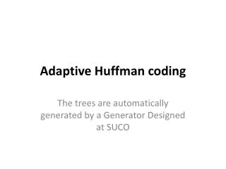
Variations • n-ary Huffman coding • Uses {0, 1, .., n-1} (not just {0,1}) • Adaptive Huffman coding • Calculates frequencies dynamically based on recent actual frequencies • Huffman template algorithm • Generalizing • probabilities any weight • Combining methods (addition) any function • Can solve other min. problems e.g. max [wi+length(ci)]
Image Compression • 2-stage Coding technique • A linear predictor such as DPCM, or some linear predicting function Decorrelate the raw image data • A standard coding technique, such as Huffman coding, arithmetic coding, … Lossless JPEG: - version 1: DPCM with arithmetic coding - version 2: DPCM with Huffman coding
DPCMDifferential Pulse Code Modulation • DPCM is an efficient way to encode highly correlated analog signals into binary form suitable for digital transmission, storage, or input to a digital computer • Patent by Cutler (1952)
Huffman Coding Algorithm for Image Compression • Step 1. Build a Huffman tree by sorting the histogram and successively combine the two bins of the lowest value until only one bin remains. • Step 2. Encode the Huffman tree and save the Huffman tree with the coded value. • Step 3. Encode the residual image.
Huffman Coding of the most-likely magnitudeMLM Method • Compute the residual histogram H H(x)= # of pixels having residual magnitude x • Compute the symmetry histogram S S(y)= H(y) + H(-y), y>0 • Find the range threshold R for N: # of pixels , P: desired proportion of most-likely magnitudes
References • MacKay, D.J.C. , Information Theory, Inference, and Learning Algorithms, Cambridge University Press, 2003. • Wikipedia, http://en.wikipedia.org/wiki/Huffman_coding • Hu, Y.C. and Chang, C.C., “A new losseless compression scheme based on Huffman coding scheme for image compression”, • O’Neal