Content Based Image Clustering and Image Retrieval Using Multiple Instance Learning Xin Chen
Content Based Image Clustering and Image Retrieval Using Multiple Instance Learning Xin Chen Advisor: Chengcui Zhang Department of Computer and Information Sciences, University of Alabama at Birmingham. 98. 98. 98. 56. 56. 56. 10. 10. 10. 23. 653. 357. 228. 469. 167.

Content Based Image Clustering and Image Retrieval Using Multiple Instance Learning Xin Chen
E N D
Presentation Transcript
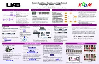
Content Based Image Clustering and Image Retrieval Using Multiple Instance Learning Xin Chen Advisor: Chengcui Zhang Department of Computer and Information Sciences, University of Alabama at Birmingham 98 98 98 56 56 56 10 10 10 23 653 357 228 469 167 Content Based Image Retrieval System Overview Image Segmentation and Feature Extraction Parents C1 and C2 Iterate K times Experiment shows cut = 2/3. Adjust according to specific problem. 23 653 357 228 469 167 823 823 Randomly Generate a Small Number r Randomly choose mutation point 23 653 966 228 469 167 823 N Y <cut r Y Y Null Null N N 30% 10% offspring C1 C3 C 4 C2 20% 40% • where u and v are two data points. We choose to use Radial Basis Function (RBF) Machine: • Mathematically, One-Class SVM solves the following quadratic problem: • subject to • where is the slack variable, and α(0,1) is a parameter that controls the trade off between maximizing the distance from the origin and containing most of the data in the region created by the hyper-sphere and corresponds to the ratio of “outliers” in the training dataset. • When it is applied to the MIL problem, It is also subject the MIL Equation. • If w and are a solution to this problem, then the decision function is • It will be 1 for most examples xi contained in the training set. • Given a query image, in initial query, the user needs to identify a semantic region of interest. Since no training sample is available at this point, we simply compute the Euclidean distances between the query semantic region and all the other semantic regions in the image database. • The similarity score for each image is then set to the inverse of the minimum distance between its regions and the query region. The training sample set is then constructed according to user’s feedback. • If an image is labeled positive, its semantic region that is the least distant from the query region is labeled positive. In this way, most of the positive regions can be identified. • For some images, Blob-world may “over-segment” such that one semantic region is segmented into two or more “blobs”. In addition, some images may actually contain more than one positive region. Suppose the number of positive images is h and the number of all semantic regions in the training set is H. Then the ratio of “outliers” in the training set is set • to: • z is a small number used to adjust the α in order to alleviate the above mentioned problem. • The training set as well as the parameter α are fed into One-Class SVM to obtain and ,which are used to calculate the value of the decision function for the test data. • Each image region will be assigned a “score” by in the decision function. The higher the score, the more likely this region is in the positive class. The similarity score of each image is then set to the highest score of all its regions. Third Query Result Retrieved Segments = × - f(x) sign(w θ(x) ρ) Clustering with Genetic Algorithm: Overview • The possible solutions to a real world problem are evaluated. Each solution is given a “score”. Then they are encoded as chromosomes and fed into Genetic World. • These chromosomes are parents or the tth generation. Genetic World operators (e.g. Selection, Crossover and Mutation) manipulate these chromosomes and generate the offspring i.e. the (t+1)th generation. When doing this, a mechanism is implemented to make sure that the higher the score the higher the chance a certain chromosome is inherited. • Offspring are decoded into real world solutions. • Evaluation in Real World is performed again upon the generated solutions. • The evaluated solutions are encoded and fed back into Genetic World for another round of evaluation. • End of iterations until a certain criteria is satisfied. • CBIR Procedure • Preprocessing: Images are segmented into a set of image instances. Features of each instance are extracted. • Clustering: Image instances are clustered to reduce the search space of the learning algorithm. • User Query: User provide a query image. • SVM Learning: One-class SVM is the similarity calculation algorithm, which learns user query and feedback and return results to the user. • Return Results: In each iteration, user give feedback to the returned results. SVM refines the retrieval results accordingly in the next iteration. Motivation The amount of image data involved is very large. We use clustering to preprocess the data and reduce the search space in image retrieval. For this reason, we choose Genetic Algorithm in the hope that the clustering result can reach global optimum. The objects in clustering are image segments. Therefore, if a certain image segment belongs to a cluster, the image that contains this object also belongs to this cluster. In this way, we can reduce the amount of image searched in the final retrieval process. • Segmentation • We use Blobworld[1] automatic image segmentation method to partition all the images in image database into several segments. Each segment represent an individual semantic region of the original image. E.g. grass, lake, deer, tree etc. • Feature Extraction • Then we extract features for each image segment. In our experiment, 8 features are used – 3 color features, 3 texture features and 2 shape features. Clustering with Genetic Algorithm: Algorithm Design Multiple Instance Learning • Key Points in Design • Encoding • Object Function • Genetic Operators: Selection, Recombination and Mutation Mutation Change a gene to an item that is not included in this chromosome at a very low frequency. Recombination Operator Selection Operator • For each item, compute its fitness (i.e. the inverse value of object function): f1, f2,…, fn. • Total fitness: • Relative fitness of each item is fi/F. It is its probability of being inherited to the next generation. • Simulate roulette to choose pairs of chromosomes that will be used to generate the next generation. In the example below, C1 on Roulette stands for Chromosome 1 whose fitness score is 30%. • Bag: Each image is a bag that has a certain number of instances. • MIL: A training sample is a labeled bag in which the labels of the instances in the bag are unknown. • In each iteration, user provides feedback to the returned images. If a image is relevant, it is labeled positive, otherwise it is labeled negative. In this way, bag (image as a whole) label is known while instance (image segments) labels are unknown. But we know the relationship between these two kinds of labels. If the bag label is positive, there exist at least one positive instance label in the bag. If the bag label is negative, all the instances are negative. This can be mathematically depicted below. Encoding For example,to partition 1000 objects into 10 clusters. Give each item an ID: 1,2,…,1000. A feasible solution is: Each integer in the allele is the ID of a centroid. • Wrap-up • At the end of clustering we have k clusters. • Given a query image region, all the other image regions in this cluster can be located. • In some cases, the query region is also very close to image regions in another cluster. • We choose three clusters whose centroids are the closest to the query region. • We then group all the images that have at least one semantic region fall into the three clusters and take it as the reduced search space . Object Function Clustering is reduced to find the optimal combination. The goal is to find a set of centroids that make the function below has its minimum: Where R is the subset of P,and it has k items. d is Euclideandistance. Different from crossover operator in simple genetic algorithm, this is to guarantee there’s no repeated genes in one chromosome, i.e. centroids in one solution are all distinct. One-Class Support Vector Machine (SVM) Experimental Results • One-Class Support Vector Machine • Motivation: Good image regions are good in the same way. But bad image regions are bad in their own way. • Basic Idea: The idea is to model the dense region as a “ball” – a hyper-sphere. In MIL problem, positive instances are inside the “ball” and negative instances are outside. • 9,800 images with 82,556 instances are used as test data. • We tested on 65 query images. The search space is reduced to 28.6% on average. • In initial query, the system gets the feature vector of the query region and compares it with all the other image regions in the database using Euclidean distance. The top thirty images are returned to the user. • After the initial query, user gives feedback to the retrieved images and these feedbacks are returned to the system. Our One-Class SVM based algorithm learns from these feedbacks and starts another round of retrieval. • Learning Procedure • Apply the strategy of Schölkopf’s One-Class SVM[2]. First do a mapping to transform the data into a feature space F corresponding to the kernel K: • Through each iteration, the number of positive images increases steadily.