Download

1 / 33
330 likes | 420 Views
This book covers the design needs and numerical approach for modeling high-frequency results in semiconductor structures. It explores the physical meaning of vector potentials and provides insights into interconnects, integrated passives, RF components, and the simulation of RF components.

E N D
Electromagnetic Modeling of Back-End Structures on Semiconductors Wim Schoenmaker
Introduction and problem definition Designer’s needs: the numerical approach Putting vector potentials on the grid Static results High-frequency results Conclusions Outline
Introduction and problem definition Designer’s needs: the numerical approach Vector potentials: their ‘physical’ meaning Static results High-frequency results Conclusions Outline
Introduction -interconnects Transistors (gates, sources and drains) On-chip connections between transistors Dimensions/pitches still decreasing Increasing clock frequencies Frequency dependent factors become more and more important: e.g. Cross-talk, skin effect, substrate currents
Introduction - integrated passives Passive structures in RF systems – e.g. antennas, switches, … Cost reduction by integration in IC’s Simulation of RF components • Increases reliability • Increases production yield • Decreases developing cycle RF section WLAN receiver - 5.2 GHz
Introduction and problem definition Designer’s needs: the numerical approach Putting vector potentials on the grid Static results High-frequency results Conclusions Outline
constraints: Use the ‘language’ of designers notelectric and magnetic fields (E,B) but Poisson field V and at high frequency also vector potential A Full 3D approach exploit Manhattan structure, i.e. 3D grid Include high frequency consideration work in frequency space provide designers with R(w), C(w), L(w),G(w) parameters (resistance R, capacitance C, inductance L, conductance G) Designer’s needs -Problem definition
Designer’s needs -numerical approach WARNING!! Engineers write:
Jn is the electron current density Jp is the hole current density U is recombination – generation term p local hole concentration n electron concentration T is lattice temperature k is Boltzmann’s constant Q is elementary charge Constitutive laws Conductors with ... gives ... V, A, n and p as independent variables Semi-conductors
Question: How to put V and A on a discrete grid ? Answer (1): V is a scalar and could be assigned to nodes Answer (2):A= (Ax,Ay,Az) and with we obtain a 3-fold scalar equation (Ax,Ay,Az) on nodes too! BUT VECTOR = 3-FOLD SCALAR Designer’s needs -numerical approach
Introduction and problem definition Designer’s needs: the numerical approach Putting vector potentials on the grid Static results High-frequency results Conclusions Outline
So far A.dx infinitesimal 1-form: On the computer dx : Dxare the distances between grid nodes i.e. connections on the grid A is a connection A exists between the grid nodes Continuum vs discrete
Equations to be solved Discretization of V is standard: V is put in nodes A is put on the links Implementation for numerical simulation Vj=V(xj ) Vi=V(xi ) Aij=A(xi ,xj )=A.em
Discretizing A Stokes theorem: Stokes theorem once more:
Now 4 times L geometrical factor Discretizing A
Grid with N3 nodes N3 unknowns (Vi) 3N3(1-1/N) links 3N3(1-1/N) unknowns (Al) N3 equations for V there are 3N3(1-1/N) equations for A BUT not all A are independent PROBLEM! # equations = # unknows Counting nodes & links & equations
Solution: Select a gauge condition Coulomb gauge Lorentz gauge …. Coulomb gauge Gauge condition Each node induces a constraint between A-variables total =N3
Old proposal: build a ‘gauge tree’ in the grid highly non-local procedure difficult to program New proposal:force # equations to match # unknowns introduce extra field such that ‘ghost’ field Implementation of gauge condition Local procedure sparse matrices easy to program N3 variables ci
Core Idea c • Old system of equations • New system of equations Ghost field
Gauge implementation So .. we do not solve But ... Sparse Local procedure creates a matrix Diagonal dominant Easy to program Regular
Gauge implementation • Exploit the fact that • We can make a Laplace operator for one-forms on the grid by • This is an alternative for the ghost field method
Introduction and problem definition Designer’s needs: the numerical approach Vector potentials: their physical meaning Classical ghosts: a new paradigm in physics Static results High-frequency results Conclusions Outline
What is a paradigm ? paradigm shift = change of the perception of the world (Thomas Kuhn) Examples Copernicus view on planetary orbits Einstein’s view on gravity ~curvature of space-time Scientific revolutions with periodicity of 1 year ? Management (pep) talk –software vs 3.4 --> vs 3.5 300 years ? Ok, see examples above 25 years ? Acceptable and operational use of the word “paradigm” Why a paradigm ?
Introduction and problem definition Designer’s needs: the numerical approach Vector potentials: their physical meaning Static results High-frequency results Outline
Spiral inductor Static B-field of ring Emagn1=1.82E-19 J Emagn2=1.87E-19 J L=3.69E-13 H Static B-field of spiral Emagn1=1.16E-12 J Emagn2=1.20E-12 J L=2.041E-11 H
Introduction and problem definition Designer’s needs: the numerical approach Vector potentials: their physical meaning Classical ghosts: a new paradigm in physics Static results High-frequency results Conclusions Outline
Results:Cylindrical wire (Al) 2 a = 3 mm 4 GHz 15 GHz 25 GHz 50 GHz 100 GHz
Analytical result Solver Results:Cylindrical wire Resistance (analytical) Resistance (solver) Reactance (analytical) Reactance (solver) GHz 4 DC 14 85 30 55
Proximity effect Current density 3 GHz 1 GHz
Problem: Alternating currents alternating fields alternating currents ….. Substrate Current
~V Results: ring • Boundary conditions: • A-field on boundary vanishes • (DC = no perp B-field) • dV/dn perp to edge of simulation domain vanishes • (DC = no perp E-field) • On the contacts a harmonic signal for V • Consider only first harmonic variables