Transfer of charged molecules

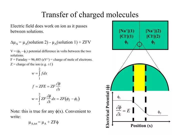
1. Transfer of charged molecules Electric field does work on ion as it passes between solutions. DµA = µA(solution 2) - µA(solution 1) + ZFV V = (f2 - f1) potential difference in volts between the two solutions. F = Faraday = 96,485 (eV-1) = charge of mole of electrons. Z = charge of the ion (e.g. ±1) Note: this is true for any f(x). Convenient to write: µA,tot = µA + ZFf [Na+](1) [Cl-](1) f1 [Na+](2) [Cl-](2) f2 f1 Electrical Potential (f) f2 Position (x)

2. Electrostatics in Water + + Counter charges (in solution) + + + + - - - - - - y = f(s) Charged surface s = charge density y Potential Chemical potentials of molecules on the surface are influenced by the surface potential, y.

3. Gouy-Chapman Theory + + LD + + + + - - - - - - y0 Potential

4. Surface Potential + + LD + + + + - - - - - - s y0 Potential Gouy Equation

5. Linearized Poisson-Boltzmann Equation + + LD + + Good for y0 ≤ 25 mV + + - - - - - - s y0 Potential

6. Mobility and Chemical Potential • Molecular motion and transport disucssed in TSWP Ch. 6. We can address this using chemical potentials. • Consider electrophoresis: • We apply an electric field to a charged molecule in water. • The molecule experiences a force (F = qE) • It moves with a constant velocity (drift velocity = u) • It obtains a speed such that the drag exactly opposes the electrophoretic force. No acceleration = steady motion. • u =qE·1/f where f is a frictional coefficient with units of kg s-1. • qE is a force with units of kg m s-2 giving u with the expected ms-1 velocity units. • Think of (1/f) as a mobility coefficient, sometimes written as µ. • u = mobility · force • We can determine the mobility by applying known force (qE) and measuring the drift velocity, u.

7. Mobility and Chemical Potential • Gradient of the chemical potential is a force. • Think about gradient of electrical potential energy: • Extending this to the total chemical potential: • where f is a frictional coefficient • (1/f) as a mobility coefficient

8. E + Mobility and Chemical Potential: Example - + Write down chemical potential as a function of position in this electrophoresis: If concentration (c) is constant througout: And the drift velocity is Potential (f) Position (x) What if c is not constant? Can the entropy term give rise to an effective force that drives motion? This is diffusion, and we can derive Fick’s Law (TSWP p. 269) from chemical potentials in this way.

9. Brownian Motion Brownian trajectory • Each vertex represents measurement of position • Time intervals between measurements constant • After time (t) molecule moves distance (d) • 2-dimensional diffusion: • <d2> = <x2> + <y2> = 4Dt • 3-dimensional diffusion: • <d2> = <x2> + <y2> + <z2> = 6Dt • In cell membrane, free lipid diffusion: • D ~ 1 µm2/s 1 “Random walk” µm t = 0 d 0 t = 0.5 s 0 1 µm A lipid will diffuse around a 10 µm diameter cell:

10. Diffusion: Fick’s First Law 1 • Jx = Flux in the x direction • Flux has units of #molecules / area • (e.g. mol/cm2) • Brownian motion can lead to a net flux of molecules in a given direction of the concentration is not constant. • Ficks First Law: µm 0 0 1 µm

11. Derivation of Fick’s First Law from Entropy of Mixing • Chemical potential of component 1 in mixture. • Net drift velocity (u) related to gradient of chemical potential by mobility (1/f) where f is frictional coefficient. • Flux (J1x) is simply concentration times net drift. • Einstein relation for the diffusion coefficient. • Entropy is the driving force behind diffusion.

12. Fick’s Second Law: The Diffusion Equation • Consider a small region of space (volume for 3D, area for 2D) • Jx(x) molecules flow in and Jx(x+dx) molecules flow out (per unit area or distance per unit time). N

13. Equilibrium Dialysis Example At equilibrium: O2(out) = O2(in, aq) [Mb·O2]/[Mb][O2(aq)] = Keq If we are able to asses the total ligand concentration in the dialysis bag: [O2(aq)] + [Mb·O2] = [O2 (in, total)] Then [Mb·O2] = [O2 (in, total)] - [O2(aq)] (these are measurable) Can compute Keq. If we have direct a probe for Mb·O2, then we don’t need the dialysis, can read of concentrations and compute Keq. Dialysis can also be used to exchange solution (eg. change [salt]) H2O (l) O2(aq), N2(aq) etc. H2O (l) O2(aq), N2(aq) Mb(aq), Mb·O2(aq) Semipermeable membrane (cellulose): allows water and dissolved small solutes to pass, blocks passage of large proteins such as myoglobin (Mb)

14. Scatchard Equation General version: M + A M·A Keq = [M·A]/([M][A]) Simplify by introducing n, the average number of ligand molecules (A) bound to the macromolecule (M) at equilibrium: Scatchard plot NKeq Slope = -Keq n/[A] Scatchard equation N independent binding sites per macromolecule. For one ligand binding site per macromolecule n N

15. Cooperative Binding For a macromolecule with multiple binding sites, binding to one site can influence binding properties of other sites. Failure of data plotted in a Scatchard plot to give a straight line indicates cooperative or anticooperative binding among binding sites. Cooperative = binding of second ligand is made easier Anticooperative = binding of second ligand is made more difficult Hemoglobin is a favorite example of a protein with cooperative binding behavior. • Binds up to 4 O2 • Cooperative: most O2 released in tissue while binding O2 maximally in the lungs • Binding curve shows characteristic sigmoidal shape 1 Myoglobin Hemoglobin f p50 = 1.5 Torr p50 = 16.6 Torr f = fraction of sites bound 0 PO2(Torr) 0 40

16. Hill Plot Scatchard equation (non-cooperative binding) For cooperative binding. n = Hill coefficient K = a constant, not the Keq for a single ligand Slope of each line give the Hill cooperativity coefficient. Slope = 1 no cooperativity Slope = N maximum (all-or-nothing) cooperativity See Example 5.4 (TSWP p. 204 - 207) for a detailed study of Hemoglobin 1.5 Myoglobin n = 1.0 log[f /(1-f)] Hemoglobin n = 2.8 -1.5 -0.5 +2 log[P02] (Torr)