IP modeling techniques II
IP modeling techniques II. In this handout, Modeling techniques: Either-Or Constraints Big M method Balance constraints Fixed Charges Applications: Multi-period production planning Inventory management. Modeling technique: Either-Or Constraints. In some situations,

IP modeling techniques II
E N D
Presentation Transcript
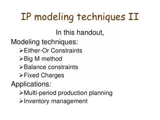
IP modeling techniques II In this handout, Modeling techniques: Either-Or Constraints Big M method Balance constraints Fixed Charges Applications: Multi-period production planning Inventory management
Modeling technique: Either-Or Constraints • In some situations, a choice can be made between two constraints, so that only one (either one) must hold whereas the other one can hold but is not required to do so. • E.g., recall the capacity constraints for the furniture manufacturer example: pine: 5xt + 1xc + 9xd 1500 (1) oak: 2xt + 3xc + 4xd 1000 (2) Suppose the furniture can be made from either pine or oak but we don’t need both. How to achieve that in the model?
Either-Or Constraints • Introduce new binary variables. For i=1,2 • Only one of (1) and (2) must hold. Thus, add a constraint: y1+y2 = 1 • We also need: y1=1 implies 5xt+1xc+9xd 1500 y2=1 implies 2xt+3xc+4xd 1000 How to express these implications by linear constraints?
Either-Or Constraints • New idea: use the big number method. • Select a huge positive number M. • Note that5xt+1xc+9xd 1500+M holds for any reasonable choices ofxt, xc, xd . It is equivalent of not putting any restriction on xt, xc, xd at all. • Consider constraint 5xt+1xc+9xd 1500+M(1-y1) (3) • If y1=1 then (3) is equivalent to (1) • If y1=0 then (3) doesn’t impose any restriction on xt, xc, xd • Thus, the set of constraints 5xt+1xc+9xd 1500+M(1-y1) 2xt+3xc+4xd 1000+M(1-y2) y1+y2 = 1 provides that only one of 5xt+1xc+9xd 1500 and2xt+3xc+4xd 1000must hold.
k out of p constraints must hold • Suppose the model includes a set of p constraints f1(x1, x2, …, xn) d1 f2(x1, x2, …, xn) d2 .... fp(x1, x2, …, xn) dp such that only some k of these constraints must hold. • Generalizing the big M method of the previous slide, that condition is achieved by the following set of constraints: f1(x1, x2, …, xn) d1+My1 f2(x1, x2, …, xn) d2+My2 …. fp(x1, x2, …, xn) dp+Myp y1+y2+…+yp = p – k y1, y2,…, yp binary
IP modeling: Multi-period production planning • A manufacturer wishes to schedule production for K periods in advance to meet known monthly demands for a given product. • Demand for period i is Di . • In period i, at most Ci items can be produced at cost $pi per item. • The demand of the current period can be satisfied by the items produced in earlier production periods (aka inventory). • The cost of holding an item in inventory from period i to period i+1 is $hi. • No inventory at the beginning of the first period. At most Hiitems are allowed in inventory at the beginning of period i. • Goal: Formulate an IP which will minimize the total cost while satisfying the demands.
IP modeling: Multi-period production planning • What variables should we have? Define xi = number of items produced in periodi , fori=1,...,k . wi= number of items in inventory at the beginning of periodi , fori=1,...,k+1 . (xi andwi are nonnegative integers) • What is the objective function? Minimize the total production and inventory cost: • Some obvious constraints. Production limit: xi Ci , fori=1,...,k Inventory limit: wi Hi, fori=1,...,k+1 No inventory before period 1: w1 = 0
Multi-period production planning: Balance Constraints • Also need constraints satisfying the demands, and relatingxi andwi . • Consider the following diagram for periodi: • The corresponding constraint for period i (i=1,…,k): wi + xi = Di + wi+1 This is known as balance constraint, and is often used in multi-period problems. Note that the balance constraints provide that wi + xi ≥ Di (sincewi+1 ≥ 0), and thus the demands are satisfied. wi Di Period i INPUT OUTPUT xi wi+1
Multi-period production planning: Complete IP model s.t. xi Ci , fori=1,...,k wi Hi, fori=1,...,k+1 wi + xi = Di + wi+1 , fori=1,…,k w1 = 0 xi ≥ 0integerfori=1,…,k wi ≥ 0 integer fori=1,...,k+1
Multi-period production planning: Fixed Setup Cost • Note that the demand of the current period can be totally satisfied by the inventory carried from the previous period. • Suppose there is a setup cost $si for period i if we decide to have any production for that period (and there is no setup cost if there is no production). • How to take the setup costs into account? • We need a new entry in the objective function: ifxi>0 then si for each period i . But this is not a linear function (because no conditions are allowed on variables).
Multi-period production planning with setup cost • To overcome the problem, introduce new variables. For i=1,...,k, • Then the setup cost is siyifor periodi . • But we also need new constraints relating xi and yi . • Idea: Use the big M method. For each i=1,...,k , add a constraint xi Myi . Why does it work? • If yi=0 then ximust be 0; • If yi=1 then there is no restriction on xi. • Note that we can take M=Ci for period i. Thus, we don’t need new constraints. Simply, replace xi Ciwithxi Ciyi . • Question: Can we haveyi=1 butxi=0 for period i ?
Multi-period production planning with setup cost • Summarizing, the modified IP model is: s.t. xi Ciyi, fori=1,...,k wi Hi, fori=1,...,k+1 wi + xi = Di + wi+1 , fori=1,…,k w1 = 0 xi ≥ 0integerfori=1,…,k wi ≥ 0 integer fori=1,...,k+1 yi binary fori=1,…,k

