Human Growth: From data to functions
370 likes | 560 Views
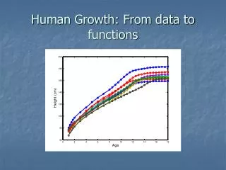
Human Growth: From data to functions. Challenges to measuring growth. We need repeated and regular access to subjects for up to 20 years. Height changes over the day, and must be measured at a fixed time.

Human Growth: From data to functions
E N D
Presentation Transcript
Challenges to measuring growth • We need repeated and regular access to subjects for up to 20 years. • Height changes over the day, and must be measured at a fixed time. • Height is measured in supine position in infancy, followed by standing height. The change involves an adjustment of about 1 cm. • Measurement error is about 0.5 cm in later years, but is rather larger in infancy.
Challenges to functional modeling • We want smooth curves that fit the data as well as is reasonable. • We will want to look at velocity and acceleration, so we want to differentiate twice and still be smooth. • In principle the curves should be monotone; i. e., have a positive derivative.
The monotonicity problem The tibia of a newborn measured daily shows us that over the short term growth takes places in spurts. This baby’s tibia grows as fast as 2 mm/day! How can we fit a smooth monotone function?
Weighted sums of basis functions • We need a flexible method for constructing curves to fit the data. • We begin with a set of basic functional building blocks φk(t), called basis functions. • Our fitting function x(t) is a weighted sum of these:
What are the main choices for basis functions? Fourier series: • a constant term, • a sine/cosine pair of fixed frequency, and • followed by a series of sine/cosine pairs with integer multiples of the base frequency. Fourier series are best for periodic data.
B-splines • These basis functions are piecewise polynomials defined by a set of discrete values called knots. • The order of the polynomials (degree + 1) controls their smoothness. • Each basis function is nonzero only over a number of contiguous inter-knot intervals equal to the order. • Polynomials are a special type of B-spline, and are thus included within the system.
When should I use B-splines? B-splines are the basis of choice for most non-periodic. • They give complete control over flexibility, allowing more flexibility where needed and less where not needed. • Computing with B-splines is extremely efficient.
Five order 2 B-spline basis functions: A basis for polygonal lines
Eight order 4 B-spline basis functions A basis for twice-differentiable functions
B-splines for growth data • We use order 6 B-splines because we want to differentiate the result at least twice. Order 4 splines look smooth, but their second derivatives are rough. • We place a knot at each of the 31 ages. • The total number of basis functions = order + number of interior knots. 35 in this case.
Isn’t using 35 basis functions to fit 31 observations a problem? • Yes. We will fit each observation exactly. • This will ignore the fact that the measurement error is typically about 0.5 cm. • But we’ll fix this up later, when we look at roughness penalties.
Okay, let’s see what happens These two Matlab commands define the basis and fit the data: hgtbasis = create_bspline_basis([1,18], 35, 6, age); hgtfd = data2fd(hgtfmat, age, hgtbasis);
Why we need to smooth Noise in the data has a huge impact on derivative estimates.
Please let me smooth the data! This command sets up 12 B-spline basis functions defined by equally spaced knots. This gives us about the right amount of fitting power given the error level. hgtbasis = create_bspline_basis([1,18], 12, 6);
These are velocities are much better. • They go negative on the right, though.
Let’s see some accelerations • These acceleration curves are too unstable at the ends. • We need something better.
A measure of roughness • What do we mean by “smooth”? • A function that is smooth has limited curvature. • Curvature depends on the second derivative. A straight line is completely smooth.
Total curvature We can measure the roughness of a function x(t) by integrating its squared second derivative. The second derivative notation is D2x(t).
Total curvature of acceleration Since we want acceleration to be smooth, we measure roughness at the level of acceleration:
The penalized least squares criterion We strike a compromise between fitting the data and keeping the fit smooth.
How does this control roughness? • Smoothing parameter λ controls roughness. • When λ= 0,only fitting the data matters. • But as λincreases, we place more and more emphasis on penalizing roughness. • As λ ∞,only roughness matters, and functions having zero roughness are used.
We can either smooth at the data fitting step, or smooth a rough function. • This Matlab command smooths the fit to the data obtained using knots at ages. The roughness of the fourth derivative is controlled. lambda = 0.01; hgtfd = smooth_fd(hgtfd, lambda, 4);
Accelerations using a roughness penalty These accelerations are much less variable at the extremes.
How did you choose λ? • We smooth just enough to obtain tolerable roughness in the estimated curves (accelerations in this case), but not so much as to lose interesting variation. • There are data-driven methods for choosing λ, but they offer only a reasonable place to begin exploring. • But smoothing inevitably involves judgment.
What about monotonicity? • The growth curves should be monotonic. • The velocities should be non-negative. • It’s hard to prevent linear combinations of anything from breaking the rules. • We need an indirect approach to constructing a monotonic model
A differential equation for monotonicity Any strictly monotonic function x(t) must satisfy a simple linear differential equation: The reason is simple: because of strict monotonicity, the first derivative Dx(t) will never be 0, and function w(t) is therefore simply D2x(t)/Dx(t).
The solution of the differential equation Consequently, any strictly monotonic function x(t) must be expressible in the form This suggests that we transform the monotone smoothing problem into one of estimating function w(t), and constants β0and β1.
What we have learned • B-spline bases are a good choice for fitting non-periodic functions; Fourier series are right for periodic situations. • We can control smoothness by either using a restricted number of basis functions, or by imposing a roughness penalty. • Roughness penalty methods generally work better. • Differential equations can play a useful role when fitting constrained functions to data.
More information • Ramsay & Silverman (1997, 2004), Chs. 3, 4, 13 • Ramsay & Silverman (2002), Ch. 6. • The long-term growth data are from the Berkeley growth study. • The infant growth data were collected by Michael Hermanussen.
Where do we go from here? • We need to look more systematically at how to smooth data. • This involves deciding what basis function system to use. • Splines are so important that we have to look at them in more detail. • Here’s a serious problem …
What’s wrong with the mean? • The cross-sectional mean is the heavy blue line. • It has less amplitude variation than any single curve. • The pubertal growth spurt for the mean lasts longer than does any single curve. • The problem is that we are averaging over curves in quite different stages of growth.
What’s wrong with the mean? • The cross-sectional mean is the heavy blue line. • It has less amplitude variation than any single curve. • The pubertal growth spurt for the mean lasts longer than does any single curve. • The problem is that we are averaging over curves in quite different stages of growth.
Phase and Amplitude Variation • Functional data like growth curves often show variation in the timing of events, like the pubertal growth spurt. • This is called phase variation. • We have to find out how to separate phase from amplitude variation before we can do even simple things like compute mean curves.