Production Functions

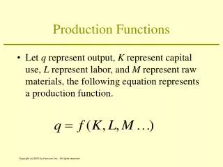
Production Functions • Let q represent output, K represent capital use, L represent labor, and M represent raw materials, the following equation represents a production function.

Marginal Physical Productivity • Marginal physical productivity is the additional output produced by adding one more unit of an input while holding all other inputs constant. • The marginal product of labor (MPL) is the extra output obtained by employing one more unit of labor holding capital constant.

Marginal Physical Productivity • The marginal product of capital (MPK) is the extra output obtained by using one more machine while holding the number of workers constant.

Diminishing Marginal Physical Product • Marginal physical product of an input will depend upon the level of the input used. • It is expected that marginal physical product will eventually diminish as shown in Figure 5.1.

FIGURE 5.1: Relationship between Output and Labor Input Holding Other Inputs Constant Total Output Output per week L* Labor input per week (a) Total Output MP L L* Labor input per week (b) Marginal Productivity

Diminishing Marginal Physical Product • The top panel of Figure 5.1 shows the relationship between output per week and labor input during the week as capital is held fixed. • Initially, output increases rapidly as new workers are added, but eventually it diminishes as the fixed capital becomes overutilized.

Marginal Physical Productivity Curve • The marginal physical product curve is simply the slope of the total product curve. • The declining slope, as shown in panel b, shows diminishing marginal productivity.

Average Physical Productivity • Average physical product is simply “output per worker” calculated by dividing total output by the number of workers used to produce the output. • This corresponds to what many people mean when they discuss productivity, but economists emphasize the change in output reflected in marginal physical product.

Appraising the Marginal Physical Productivity Concept • Marginal physical productivity requires the ceteris paribus assumption that other things, such as the level of other inputs and the firm’s technical knowledge, are held constant. • An alternative way, that is more realistic, is to study the entire production function for a good.

Isoquant Maps • An isoquant is a curve that shows the various combinations of inputs that will produce the same amount of output. • The curve labeled q = 10 is an isoquant that shows combinations of labor and capital, such as points A and B, that produce exactly 10 units of output per period

FIGURE 5.2: Isoquant Map Capital per week KA A q = 30 q = 20 KB B q = 10 0 Labor per week LA LB

Rate of Technical Substitution • Theslope of an isoquant is called the marginal rate of technical substitution (RTS), the amount by which one input can be reduced when one unit of another input is added. • It is the rate that capital can be reduced, holding output constant, while using one more unit of labor.

Rate of Technical Substitution

Diminishing RTS • Along any isoquant the (negative) slope become flatter and the RTS diminishes. • When a relatively large amount of capital is used (as at A in Figure 5.2) a large amount can be replaced by a unit of labor, but when only a small amount of capital is used (as at point B), one more unit of labor replaces very little capital.

Returns to Scale • Returns to scale is the rate at which output increases in response to proportional increases in all inputs. • In the eighteenth century Adam Smith became aware of this concept when he studied the production of pins.

Returns to Scale • Adam Smith identified two forces that come into play when all inputs are increased. • A doubling of inputs permits a greater “division of labor” allowing persons to specialize in the production of specific pin parts. • This specialization may increase efficiency enough to more than double output. • However these benefits might be reversed if firms become too large to manage.

Constant Returns to Scale • A production function is said to exhibit constant returns to scale if a doubling of all inputs results in a precise doubling of output. • This situation is shown in Panel (a) of Figure 5.3.

Decreasing Returns to Scale • If doubling all inputs yields less than a doubling of output, the production function is said to exhibit decreasing returns to scale. • This is shown in Panel (b) of Figure 5.3.

Increasing Returns to Scale • If doubling all inputs results in more than a doubling of output, the production function exhibits increasing returns to scale. • This is demonstrated in Panel (c) of Figure 5.3. • In the real world, more complicated possibilities may exist such as a production function that changes from increasing to constant to decreasing returns to scale.

FIGURE 5.3: Isoquant Maps showing Constant, Decreasing, and Increasing Returns to Scale A A Capital Capital per week per week 4 4 q = 40 3 q = 30 3 q = 30 2 2 q = 20 q = 20 1 1 q = 10 q = 10 Labor Labor 0 1 2 3 4 0 1 2 3 4 per week per week (a) Constant Returns to Scale (b) Decreasing Returns to Scale A Capital per week 4 3 q = 40 2 q = 30 q = 20 1 q = 10 Labor 0 1 2 3 4 per week (c) Increasing Returns to Scale

APPLICATION 5.3: Returns to Scale in Beer Brewing • Economies to scale were achieved through automated control systems in filling beer cans. • National markets foster economies of scale in distribution and advertising (especially television). • These factors became especially important after World War II and the number of U.S. brewing firms fell by over 90 percent between 1945 and the mid-1980s.

APPLICATION 5.3: Returns to Scale in Beer Brewing • The industry consolidated with a few firms operating large breweries in multiple locations to reduce shipping costs. • Beginning the 1980s, smaller firms offering premium brands, provided an opening for local microbreweries. • A similar event occurred in Britain in the 1980s with the “real ale” movements, but it was followed by small firms being absorbed by national brands. • A similar absorption may be starting to take place in the United States.

Input Substitution • Another important characteristic of a production function is how easily inputs can be substituted for each other. • This characteristic depends upon the slope of a given isoquant, rather than the whole isoquant map.

Fixed-proportions Production Function • It may be the case that absolutely no substitution between inputs is possible. • This case is shown in Figure 5.4. • If K1 units of capital are used, exactly L1 units of labor are required to produce q1 units of output.

FIGURE 5.4: Isoquant Map with Fixed Proportions Capital per week A K2 q2 K1 q1 q0 K0 0 Labor per week L0 L1 L2

Fixed-proportions Production Function • This type of production function is called a fixed-proportion production function because the inputs must be used in a fixed ratio to one another. • Many machines require a fixed complement of workers so this type of production function may be relevant in the real world.

The Relevance of Input Substitutability • Over the past century the U.S. economy has shifted away from agricultural production and towards manufacturing and service industries. • Economists are interested in the degree to which certain factors of production (notable labor) can be moved from agriculture into the growing industries.

Changes in Technology • Technical progress is a shift in the production function that allows a given output level to be produced using fewer inputs. • In studying productivity data, especially data on output per worker, it is important to make the distinction between technical improvements and capital substitution.

APPLICATION 5.4: Multifactor Productivity • Table 1 shows the rates of change in productivity for three countries measured as output per hour. • While the data show declines during the 1974 to 1991 period, they still averaged over 2 percent per year. • However, this measure may simply reflect simple capital-labor substitution.

APPLICATION 5.4: Multifactor Productivity • A measure that attempts to control for such substitution is called mutifactor productivity. • As table 2 shows, the 1974 - 91 period looks much worse using the multifactor productivity measure.

APPLICATION 5.4: Multifactor Productivity • Reasons for the decline in post 1973 productivity include rising energy prices, high rates of inflation, increasing environmental regulations, deteriorating education systems, or a general decline in the work ethic. • Clearly after 1991, productivity has improved greatly.

TABLE 1: Annual Average Change in Output per Hour in Manufacturing

TABLE 2: Annual Average Change in Multifactor Productivity Manufacturing

A Numerical Example • Assume a production function for the fast-food chain Hamburger Heaven (HH): - where K represents the number of grills used and L represents the number of workers employed during an hour of production.

TABLE 5.1: Hamburger Production Exhibits Constant Returns to Scale

Average and Marginal Productivities • Holding capital constant (K = 4), to show labor productivity, we have • Table 5.2 shows this relationship and demonstrates that output per worker declines as more labor is employed.

TABLE 5.2: Total Output, Average Productivity, and Marginal Productivity with Four Grills

The Isoquant Map • Suppose HH wants to produce 40 hamburgers per hour. Then its production function becomes

TABLE 5.3: Construction of the q = 40 Isoquant

Technical Progress • Technical advancement can be reflected in the equation • Comparing this to the old technology by recalculating the q = 40 isoquant

FIGURE 5.6: Technical Progress in Hamburger Production Grills (K) 10 4 q = 40 before invention q = 40 1 4 10 Workers (L)

Production Functions