Download
1 / 50
500 likes | 672 Views
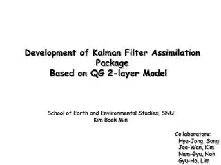
Development of Kalman Filter Assimilation Package Based on QG 2-layer Model . School of Earth and Environmental Studies, SNU Kim Baek Min. Collaborators: Hyo-Jong, Song Joo-Wan, Kim Nam-Gyu, Noh Gyu-Ho, Lim. Today’s talk. Review the current status of EnKF

E N D
Development of Kalman Filter Assimilation Package Based on QG 2-layer Model School of Earth and Environmental Studies, SNU Kim Baek Min Collaborators: Hyo-Jong, Song Joo-Wan, Kim Nam-Gyu, Noh Gyu-Ho, Lim
Today’s talk • Review the current status of EnKF • Exploration of world of EnKF with Lorenz model • Description of Lorenz QG 2-layer model • EnKF test with QG model • (If you are not still hungry or not still bored^^;) • Introduction to New Efficient EKF
Current status of EnKF • Many centers still use 3D-Var though it can not represent time-varying error statistics. • Several centers (ECMWF, UK, Canada) have switched to 4D-Var, better than 3D-Var. • 4D-Var was clearly better than 3D-Var, but EnKF was only comparable to 3D-Var (Mitchell and Houtekamer,2003). • Whitaker and Hamill(2005) show EnKF better than NCEP’s 3D-Var for real data. • Houtekamer and Mitchell(2005) show that EnKF is now as good as 4D-Var.
Traditional OI Analysis equation • There is no model for covariance • Forecast covariance matrix should be given apriori • Observation error is represented by: • transforms from model space to obs. space
Traditional Kalman Filter Analysis equation(just same with OI) • Forecast is provided by integration of L with analysis • There is model for covariance • Covariance is updated with the aid of Model L • Model L should be linear model in Kalman filter
Extended Kalman Filter Analysis equation(just same with OI) • Forecast is provided by integration of N with analysis • There is model for covariance • Covariance is updated with the aid of TLM of NL • Model N is nonlinear model in Kalman filter
Interpretation of OI analysis • Given observation( ) , forecast ( ), • find the conditional probability(a posteriori prob.) through Bayes theorem. • Then, we get final analysis( ) by taking point maximizing that pdf. • The conditional probability is given by • When both obs. and forecast are unbiased! • The structure of is solely determined by • The structure of is solely determined by • When both PDF of obs. And forecast are gaussian!
Introducing Ensemble • Consider ensemble of forecast vector and observation vector: • Apply Kalman filter eq. for each jth ensemble member :
Heart of EnKF(1) • Flow dependent forecast covariance through the benefit from the well • distributed forecast ensemble members. • No more predefinition of forecast covariance except for the I.C. • Now, forecast model has ability to produce its own error statistics. • Forecast PDF follows Focker–planck equation(FPE) theoretically. • Direct linear approximation to FPE = EKF (Need TLM) • Monte-carlo approximation to FPE = EnKF(No need for TLM)
Heart of EnKF(2) • Not essential for obtaining best estimate(analysis). • But, helps to improve the spreading of analysis variance of analysis • (Burgers et al., 1998) • If ensemble is small, however, this is source of errorneous analysis • Finally, the ananlysis equation for EnKF is given by:
Interpretation of EnKF analysis approximates second mom. of approximates second mom. of
Application to Lorenz Model • Suppose we conduct EnKF assimilation applied to Lorenz model • Lorenz model • Dimension of model space is three • Dynamics of the model considerably differs depending on parameter r • r=21:Stable point attractor • r=28: Chaotic attractor
Matrix representation of EnKF(1) (Evensen, 2003) • Dimension of Model state is 3 and 100 ensemble members are used.
Matrix representation of EnKF(2) (Evensen, 2003) for our experiment.
Ensemble of 100 analysis Ensemble of 100 Forecast Statistics of Ensemble Ensemble of 100 Obs. Measurement of Obs. Integration with model Statistics of Ensemble Random generator Gaussian, Normal PDF Summary of EnKF analysis Weighted Mean
Makefile FC = pgf90 FCFLAGS = -Mfree -O2 -r8 .SUFFIXES= .F .i .o .f .f.o: $(FC) -c $(FCFLAGS) $*.f OBJS = m_multa.o random.o EnKF.o analysis.o lorzrk.o rk4.o EnKF.exe: $(OBJS) $(FC) -o $@ $(OBJS) $(FCFLAGS) ../../lib/lapack_LINUX.a ../../lib/blas_LINUX.a $(RM) $(OBJS) $(RM) *.mod clean: $(RM) EnKF.exe • analysis.f is obtained from http://www.nrsc.no/Code/ • LAPACK, BLAS is obtained from http://netlib.org
Experiment 1(Chaotic regime) • Time step=0.01 • Analysis time=every 0.5(every fifty step) • Chaotic model regime( r=28) • Assume true trajectory (x=1.5,y=-1.5,z=25.5) • Observations are simulated by adding std. dev. 1 perturbation (gauss pdf). • to true trajectory at every analysis time(OSSE)
Experiment 2(Stable regime) • Time step=0.01 • Analysis time=every 0.5(every fifty step) • Stable model regime( r=21) • Assume true trajectory (x=1.5,y=-1.5,z=25.5) • Observations are simulated by adding std. dev. 5 perturbation (gauss pdf). • to true trajectory at every analysis time(OSSE) • Model dynamics converges to stable equilibrium point. • Henceforth, cloud of model ensemble should be shrink as analysis goes by… • We still expect good result even though we provide quite bad obs(std. dev.=5).
Characteristics • Beta plane, channel • Fourier basis • Exact calculation of nonlinear terms using interaction coefficient method • (exact but slow compared to Transform method) • Runge-Kutta 4th order time integration scheme • Periodic boundary condition in west/east direction • No mass flux across the lateral boundary • Model can be as simple as possible to Lorenz 3variable model. • Model can be run in a very high resolution mode.
Friction at the interface Radiative equilibrium mean potential temperature (θ*(x,y)) Radiative cooling ρ1 ρ2 H 5000km Ekman friction 10000km Schematics
Baroclinic eddy simulation From Master thesis of Joo-Wan, Kim
Tangent Linear Model • For the development of EKF of QG model, TLM of QG model is needed. • Multi-variable taylor expansion is given by: • TLM is defined as:
Example of Tangent Linearization Basis expansion converts PDE ->ODE
Model History • Kim(Baek Min) implemented QG-2layer model based on Cehelsky and Tung(1987). • He used the model in his master thesis for the predictability study(2001). • Kim(Joo Wan) made a TLM version and obtained a singular vector of • QG-2layer model in his master thesis(2003). • Noh(Nam Kyu) implemented EKF of QG-2layer model. • He compared 4Dvar and EKF in his master thesis using Lorenz model(2005). • Song(Hyo Jong) implemented EnKF of QG-2layer model.
Estimate of the Forecast Error Covariance with Governing Eigen-modes • The forecast error covariance matrix consists of eigen-values and eigenvectors. • To estimate a variance of each eigen-mode, we need statistically 100 ensemble members. • The number of eigen-modes, which can be detected by forecast ensemble, is equal to that of ensemble members.
Estimate of the Forecast Error Covariance with Governing Eigen-modes • If the number of governing eigen-modes is smaller than 100, the forecast error covariance may be estimated by another method to reduce computational cost.
Estimate of the Forecast Error Covariance with Governing Eigen-modes