Download
1 / 21
210 likes | 406 Views
Earthquake source modelling by second degree moment tensors . Petra Adamo vá Jan Šílený. Geophysical Institute, Academy of Sciences, Prague, Czech Republic e-mail: adamova@ig.cas.cz, fax: +420-272761549. Introduction, motivation. Finite source parameters from point source approximation.

E N D
Earthquake source modelling by second degree moment tensors Petra Adamová Jan Šílený Geophysical Institute, Academy of Sciences, Prague, Czech Republic e-mail: adamova@ig.cas.cz, fax: +420-272761549
Introduction, motivation • Finite source parameters from point source approximation • traditional modeling of slip on fault plane is more complicated • 2nd degree moments are adventageous alternative • size of the source, duration of the source process, average slip on the fault, etc.
Theory: second degree moment tensors First degree moment tensor representation: Second degree moment tensor representation (Taylor expansion up to degree two):
Second degree moments, Doornbos (1982) Standard MT 1. Time derivative of the response function (1 parameter): temporal centroid – origin time of the finite extent source estimate • Spatial derivative (3 parameters): spatial centroid position • Combination of temporal and spatial derivative (3 parameters) • Second time derivative (1 parameter): source duration • From 3 and 4: rupture propagation along the fault • Second spatial derivative (6 parameters): geometrical characteristics of the source (source ellipsoid)
Application for better estimate of mechanism • High non-DC component is reported for some strong events by seismological agencies (Harvard, USGS, SED) • This component is often questionable (large events, tectonic origin) it can be false due to unmodeled source finiteness • (strong event is modeled as point source) • the scalar moment underestimation in the agency solution we will try to verify this hypothesis using synthetic test
T P N Example of high non-DC component Izmit earthquake: agency solution (ETH) Date/Time: 99/ 8/17 0: 1:38 Latitude 40.640 Longitude 29.830 Mw= 7.52 Strike = 90 Dip = 72 Rake = -164 DC = 59 % CLVD = 41 % ISO = 0 % Very high non-DC component
Synthetic test: configuration • Green’s functions are computed by DWN method • crustal model is identical for data and synthetics (Bulut et al., 2007) • noise-free data
Rupture model (J. Burjánek) Unilateral rupture Fault size: 20 km x 10 km Scalar seismic moment: 1e18 Nm f = 0 - 2 Hz Rupture velocity 2.8 km/sec
Inversion scheme Additional constraint: the volume of the focus is non-negative (McGuire et al., 2001, 2002)
Synthetic data unfiltered synthetic data demonstrating the source directivity: station SDL: direction perpendicular to the fault strike. station HER: ‘reverse’ direction station BAL: ‘forward’ direction
Results: exact data Common MT, f = 0.02 - 0.08 Hz (3rd order Butterworth filter) Theoretical mechanism Strike = 93 Dip = 73 Rake = -178 DC = 78 % CLVD = 12 % V = 10 % Strike = 90 Dip = 72 Rake = 180 DC = 100 % CLVD = 0 % V = 0 % P T N
Frequency test • low-pass filtering as much as possible: • low-pass 3rd order Butterworth filter with a low-cut off at 0.02 Hz • high-pass filter as much as possible but to keep the 2nd • degree effects • high-pass 3rd order Butterworth filter with a cut off at 0.1, 0.2, 0.3 and 0.4 Hz
Geometrical characteristics Second spatial derivative, 6 parameters A – 0.1 Hz B – 0.2 Hz C – 0.3 Hz D – 0.4 Hz frequencies used in the inversion of 2nd degree moments Optimum frequency range is up to 0.2 Hz
P T T P N N MT refinement: exclusion of 2nd degree terms Refined MT: common MT without second degree terms Strike =93 Dip = 73 Rake =2 DC = 94 % CLVD = 4% V = 2 % Strike =93 Dip = 73 Rake =2 DC = 78 % CLVD = 12 % V = 10 % Strike = 90 Dip = 72 Rake = 180 DC = 100 % CLVD = 0 % V = 0 % Theoretical mechanism
Reconstructed mechanisms 0.02- 0.1 Hz 0.02-0.2 Hz 0.02-0.08 Hz 0.02-0.08 Hz 0.02-0.08 Hz 0.02-0.3 Hz 0.02-0.08 Hz 0.02-0.4 Hz Left: the mechanism obtained by inverting data filtered outside 0.02 -0.08 Hz Right: mechanism from data corrected for the contribution of the 2nd degree moments frequency used in the inversion of 2nd degree moments
Test of robustness Experiments simulating inconsistencies during the data inversion • source mislocation (1 km E, 1 km S, 2 km Z) • larger error in depth than in the horizontal coordinates simulates smaller location precision • inaccurate GF (less layers + deviation 10% in each layer) • dashed line – simplified model • noise in data (15 - 30% from the maximal amplitude)
Geometrical characteristics Second spatial derivative, 6 parameters Bold line – exact data A - mislocation of the hypocenter when evaluating Green’s function B - mismodeling of the velocity profile: the true 1-D model used to synthesize the data, simplified when evaluating Green’s function C - noisy data
Propagation vectors exact data (black) (a) hypocenter mislocation (b) the seismic velocity profile mismodeling (c) noisy data Background: vertical projection of the source model: the moment density distribution of the unilaterally propagating rupture together with the 1 s, 2 s and 3 s isochrones.
Reconstructed mechanisms Left: the mechanism obtained by inverting data filtered outside 0.02 - 0.08 Hz Right: mechanism from data corrected for the contribution of the 2nd degree moments
Synthetic data vs. synthetic seismograms Black: synthetic data Upper gray: synthetic seismograms Lower gray: 2nd degree terms station SDL: direction perpendicular to the fault strike. station HER: ‘reverse’ direction station BAL: ‘forward’ direction Frequency range 0.02 -0.2 Hz
Conclusions • We removed false non-DC component from the data • Scalar seismic moment is higher with 2nd term than with only 1st degree term • Method of the second degree moments is perspective for applications