Lecture 17: Regression for Case-control Studies

1. Lecture 17:Regression for Case-control Studies BMTRY 701 Biostatistical Methods II

2. Old business: Comparing AUCs • Good reference: Hanley and McNeill “Comparing AUCs for ROC curves based on the same data” See class website for pdf.

3. Additional Reading in Logistic REgression • Hosmer and Lemeshow, Applied Logistic Regression • http://en.wikipedia.org/wiki/Logistic_regression • http://luna.cas.usf.edu/~mbrannic/files/regression/Logistic.html • http://www.statgun.com/tutorials/logistic-regression.html • http://www.bus.utk.edu/stat/Stat579/Logistic%20Regression.pdf • Etc: Google “logistic regression”

4. Case Control Studies in Logistic Regression • http://www.oxfordjournals.org/our_journals/tropej/online/ma_chap11.pdf • How is a case-control study performed? • What is the outcome and what is the predictor in the regression setting?

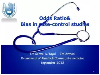
5. Recall the simple 2x2 example • Odds ratio for 2x2 table can be used in case-control studies • Similarly, the logistic regression model can be used treating ‘case’ status as the outcome. • It has been shown that the results do not depend on the sampling (i.e., cohort vs. case-control study).

6. Example: Case control study of HPV and Oropharyngeal Cancer • Gillison et al. (http://content.nejm.org/cgi/content/full/356/19/1944) • 100 cases and 200 controls with oropharyngeal cancer • How was the sampling done?

7. Data on Case vs. HPV > table(data$hpv16ser, data$control) 0 1 0 186 43 1 14 57 > epitab(data$hpv16ser, data$control) $tab Outcome Predictor 0 p0 1 p1 oddsratio lower upper p.value 0 186 0.93 43 0.43 1.00000 NA NA NA 1 14 0.07 57 0.57 17.61130 8.99258 34.49041 4.461359e-21

8. Multiple Logistic Regression • This is not ‘randomized’ study • there are lots of other predictors that may be associated with the cancer • Examples: • smoking • alcohol • age • gender

9. Fit the model: • Write down the model • assume main effects of tobacco, alcohol and their interaction • What is the likelihood function? • What are the MLEs?

10. How do we interpret the results? • Is there an effect of tobacco? • Is there an effect of alcohol? • Is there an interaction?

11. Interpreting the interaction • What is the OR for smoker/non-drinker versus a non-smoker/non-drinker? • What is the OR for a smoker/drinker versus a non-smoker/drinker?

12. How can we assess if the effect of smoking differs by HPV status?

13. How likely is it that someone who smokes and drinks will get oropharyngeal cancer? • How can we estimate the chance?

14. Matched case control studies • References: • Hosmer and Lemeshow, Applied Logistic Regression • http://staff.pubhealth.ku.dk/~bxc/SPE.2002/Slides/mcc.pdf • http://staff.pubhealth.ku.dk/~bxc/Talks/Nested-Matched-CC.pdf • http://www.tau.ac.il/cc/pages/docs/sas8/stat/chap49/sect35.htm • http://www.ats.ucla.edu/stat/sas/library/logistic.pdf (beginning page 5)

15. Matched design • Matching on important factors is common • OP cancer: • age • gender • Why? • forces the distribution to be the same on those variables • removes any effects of those variables on the outcome • eliminates confounding

16. 1-to-M matching • For each ‘case’, there is a matched ‘control • Process usually dictates that the case is enrolled, then a control is identified • For particularly rare diseases or when large N is required, often use more than one control per case

17. Logistic regression for matched case control studies • Recall independence • But, if cases and controls are matched, are they still independent?

18. Solution: treat each matched set as a stratum • one-to-one matching: 1 case and 1 control per stratum • one-to-M matching: 1 case and M controls per stratum • Logistic model per stratum: within stratum, independence holds. • We assume that the OR for x and y is constant across strata

19. How many parameters is that? • Assume sample size is 2n and we have 1-to-1 matching: • n strata + p covariates = n+p parameters • This is problematic: • as n gets large, so does the number of parameters • too many parameters to estimate and a problem of precision • but, do we really care about the strata-specific intercepts? • “NUISANCE PARAMETERS”

20. Conditional logistic regression • To avoid estimation of the intercepts, we can condition on the study design. • Huh? • Think about each stratum: • how many cases and controls? • what is the probability that the case is the case and the control is the control? • what is the probability that the control is the case and the case the control? • For each stratum, the likelihood contribution is based on this conditional probability

21. Conditioning • For 1 to 1 matching: with two individuals in stratum k where y indicates case status (1 = case, 0 = control) • Write as a likelihood contribution for stratum k:

22. Likelihood function for CLR Substitute in our logistic representation of p and simplify:

23. Likelihood function for CLR • Now, take the product over all the strata for the full likelihood • This is the likelihood for the matched case-control design • Notice: • there are no strata-specific parameters • cases are defined by subscript ‘1’ and controls by subscript ‘2’ • Theory for 1-to-M follows similarly (but not shown here)

24. Interpretation of β • Same as in ‘standard’ logistic regression • β represents the log odds ratio comparing the risk of disease by a one unit difference in x

25. When to use matched vs. unmatched? • Some papers use both for a matched design • Tradeoffs: • bias • precision • Sometimes matched design to ensure balance, but then unmatched analysis • They WILL give you different answers • Gillison paper

26. Another approach to matched data • use random effects models • CLR is elegant and simple • can identify the estimates using a ‘transformation’ of logistic regression results • But, with new age of computing, we have other approaches • Random effects models: • allow strata specific intercepts • not problematic estimation process • additional assumptions: intercepts follow normal distribution • Will NOT give identical results

27. . xi: clogit control hpv16ser, group(strata) or Iteration 0: log likelihood = -72.072957 Iteration 1: log likelihood = -71.803221 Iteration 2: log likelihood = -71.798737 Iteration 3: log likelihood = -71.798736 Conditional (fixed-effects) logistic regression Number of obs = 300 LR chi2(1) = 76.12 Prob > chi2 = 0.0000 Log likelihood = -71.798736 Pseudo R2 = 0.3465 ------------------------------------------------------------------------------ control | Odds Ratio Std. Err. z P>|z| [95% Conf. Interval] -------------+---------------------------------------------------------------- hpv16ser | 13.16616 4.988492 6.80 0.000 6.26541 27.66742 ------------------------------------------------------------------------------

28. . xi: logistic control hpv16ser Logistic regression Number of obs = 300 LR chi2(1) = 90.21 Prob > chi2 = 0.0000 Log likelihood = -145.8514 Pseudo R2 = 0.2362 ------------------------------------------------------------------------------ control | Odds Ratio Std. Err. z P>|z| [95% Conf. Interval] -------------+---------------------------------------------------------------- hpv16ser | 17.6113 6.039532 8.36 0.000 8.992582 34.4904 ------------------------------------------------------------------------------

29. . xi: gllamm control hpv16ser, i(strata) family(binomial) number of level 1 units = 300 number of level 2 units = 100 Condition Number = 2.4968508 gllamm model log likelihood = -145.8514 ------------------------------------------------------------------------------ control | Coef. Std. Err. z P>|z| [95% Conf. Interval] -------------+---------------------------------------------------------------- hpv16ser | 2.868541 .3429353 8.36 0.000 2.1964 3.540681 _cons | -1.464547 .1692104 -8.66 0.000 -1.796193 -1.1329 ------------------------------------------------------------------------------ Variances and covariances of random effects ------------------------------------------------------------------------------ ***level 2 (strata) var(1): 4.210e-21 (2.231e-11) ------------------------------------------------------------------------------ OR = 17.63