Lecture 10: Predation
Lecture 10: Predation. EEES 3050. The Nature of Predation. Types of predators predators: eat other living organisms taxonmic and functional classifications true predators Herbivores or grazers parasites Parasitoids Cannibals . Classifications. true predators: kill living prey,

Lecture 10: Predation
E N D
Presentation Transcript
Lecture 10: Predation EEES 3050
The Nature of Predation • Types of predators • predators: eat other living organisms • taxonmic and functional classifications • true predators • Herbivores or grazers • parasites • Parasitoids • Cannibals
Classifications • true predators: • kill living prey, • Need more prey/lifetime (lions, tigers and bears) • Herbivores or grazers: • small amounts of living prey • Need less prey/lifetime (ungulants, leeches, mosquitos)
Classifications • parasites: • small amounts of living prey • 1 or few prey/lifetime (aphids, flukes, worms) • parasitoids: • kill living prey • 1 per lifetime • developmental stage (wasps, nematodes) • Cannibalism • Eating others of same species • Sexual cannibalism (praying mantis) • Size-Structured (found in ~90% of aquatic species)
Predation as a process • Effect distribution • Influence the structure of a community • Top down effects • Predation as selective force • Predator-prey coevolution • Red-queen hypothesis.
Models of predation • Discrete generations: • Need to understand, but won’t explain in class. • Based on previous models with addition of predator term. • Continuous • Lotka-Voltera – again modified previous equations • Found to be too simplistic • Rosenzweig – MacArthur model.
You are responsible for – from book. • Lab studies of predation • Are there ever systems where a prey and predator establish an equilibrium in the lab? • What about oscillations. • Field studies of predation • Do predators actually impact prey populations? • What are the four responses of predators to an increase in prey populations as predicted by Holling?
You are responsible for – from book. • Optimal foraging theory. • What are the primary factors in determining what prey items a predator eats, i.e. how do you determine the profitability of a prey type? • What is the difference between a specialist and generalist predator? And how does this relate to optimal foraging models
Examine Article • Does dingo predation control the densities of kangaroos and emus? • By G. Caughley, G. C. Grigg, J. Caughley and G. J. E. Hill
Structure of research… • Observations • Hypotheses • Developed from existing theory • Experiment • Results • Discussion
What are the 3 observations? • Read the 1st four paragraphs: • Stop at the first figure:
3 paradoxical observations • Red Kangaroo density in 1975 in New South Wales is vastly greater than it was in 1845. • In South Australia the number of kangaroos appears to have remained constant. • Densities of kangaroos much lower in South Australia and Queensland compared to New South Wales • Local opinion was that kangaroos just avoided the fence. • Densities of dingoes is opposite of kangaroos.
Develop questions/hypotheses: • What are some of your hypotheses or questions?
Develop questions/hypotheses: • What were the questions developed by authors? • Read rest of introduction.
How did they test their questions? • Read Methods: • Don’t worry too much about Analysis section.
Is this a “true” experiment? • They did not manipulate anything.
Results • 1st New South Wales – South Australia
Results: NSW vs. SA • What is variance? • In the analysis… the States account for 77% of the variance in the data. • What does this mean?
Results • Read Queensland-South Australia
Results: QLD vs. SA • No significant difference.
Results • Read New South Wales – Queensland (far west)
Results • Read New South Wales – Queensland (central west)
Discussion • Read Discussion to middle of page 10
Discussion points: • The finding that the density differences between States hold 40 km from the border rules out explanation of the contrast by any local fence effect. • The difference has something to do with environmental conditions specific to the States • What about shooting of kangaroos or water sources?
Discussion points: • leaves only two hypotheses that we consider credible: • that the density contrasts reflect differing vegetations • differing rates of predation by dingoes. • Read rest of pg 10 and 1st paragraph of 11. • Looked at changes in vegetation with satellite imagery. • What did they find?
Discussion points: • What is going on in the mid west? • Read rest of discussion. • Direct interpretation: • The primitive densities of red kangaroos is kept low by dingo predation.
This study has documented a phenomenon but has not revealed a cause. We have presented and discarded several hypotheses to account for the reported contrasts in density, and are left with only one-the distribution pattern reflects different levels of predation by dingoes.
Ties to theory! • A predator usually cannot force the prey to very low density because its own numbers will decrease reciprocally as its food supply declines. • Remember Rosenzwieg-MacArthur models. • That tight dynamic is uncoupled when the prey comprises more than one species.
Ties to theory! • How can multiple prey result in low density of one prey? • if the threatened prey is taken at a higher rate than alternative prey its numbers will be lowered disproportionately. • if its intrinsic rate of increase is significantly lower than that of alternative prey • We suspect that the second mechanism is in play when dingoes prey upon kangaroos in the presence of rabbits
Final thoughts on article: • Sometimes ecology feels like quantifying the obvious. • Doesn’t mean it is easy. • On the other hand, sometimes the “obvious” isn’t quite so clear. • At the time current expectations were that predators could not impose such a large effect. • Still could be other mechanisms – no one has thought of them yet.
Evolution of predator-prey systems • Predation can be a strong selective process. • How have predators adapted to be more efficient? • How have prey adapted to stay alive?