CONFOCAL MICROSCOPY IN A NEW LIGHT

1. CONFOCAL MICROSCOPY IN A NEW LIGHT

2. Introduction to Confocal Microscopy Title: Introduction to Confocal Microscopy Presented by: Dr. Andrew Dixon Date: May 2009

3. An Introduction to Confocal Microscopy • What is the problem? • Marvin Minsky’s idea • The confocal principle • The power of confocal imaging • Increasing imaging speed • Imaging in 3-D • Summary of key points

4. What is the Problem? Optical microscope images contain both in-focus and out-of-focus detail How can one produce an image which only includes the in-focus detail?

5. All-in-Focus True color information in 3D topography Bump dimension: 13.8 µm height and 79 µm width

6. Marvin Minsky’s Idea Instead of collecting the complete image at one time, Minsky proposed to build up the image ‘point by point’. In this way one can introduce additional optical components in the light collection path to block the out-of-focus light from contributing to the image. Marvin Minsky Inventor of the confocal microscope Harvard (1955) US Patent 3,013,467

7. detector Confocal aperture illumination X X/Y Image Y Focus Cone Specimen sample The Confocal Principle The sample is illuminated with a focused spot of light. Light from the sample is re-focused at the confocal aperture. Only in-focus signal reaches the detector

8. The Optical Section Optical section ‘thickness’ depends on objective lens NA. Lateral and axial resolution are related.

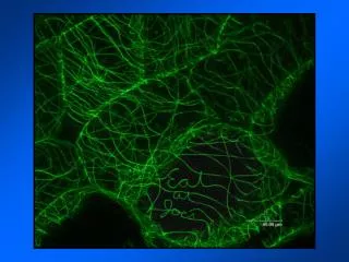
9. The Power of Confocal Imaging Conventional image In the mid 80’s mirror scanning systems were developed that adapted a conventional microscope for confocal imaging. Scientists became very excited by the images they could obtain, without having to prepare very thin section samples. (Dr. W.B. Amos, MRC Cambridge) Confocal image Bio-Rad MRC-500 Example images show tubulin structure in fertilized sea urchin egg immuno-labelled for fluorescence contrast. (scale bar 50 micron)

10. Increasing Imaging Speed Scanning a focused illumination spot, point by point is relatively slow. Several alternative schemes have been developed to increase imaging speed. One approach is to illuminate the sample simultaneously with multiple spots of light. Another approach is to illuminate the sample with a focused line of light. This is the system used in the Axio CSM 700 from Carl Zeiss.

11. From Optical Section to 3-D image A series of optical section images can be combined into a single ‘all in focus’ image, or manipulated to provide quantitative information about surface profile, surface roughness etc.

12. …A World of Possibilities Biological Research Material Sciences Neurons in a Brainbow transgenic mouse, labeled with multiple hues of fluorescent proteins. Extended focus image True color information in 3D topography Surface profiling. Surface roughness (Dr. J. Livet Harvard University)

13. In Conclusion… • Exceptional contrast optical section images • Non-contact probing and profiling • Not restricted to single color imaging • Imaging at high speed • Qualitative and quantitative 3-D characterization • High resolution surface profiling Confocal microscopy delivers…

14. End

15. Advanced Confocal Microscopy: Axio CSM 700 Title: Advanced Confocal Microscopy: Axio CSM 700 Presented by: Dr. Franz Reischer Date: May 2009

16. Axio CSM 700 – System Overview Xe illuminator, conf. microscope, controller, user PC

17. 1 2 5 3 4 Innovative Confocal Method • Xe illuminator • Multi slit grid for scanning instead of scan mirrors • Beam splitter • Sample / focal plane • Digital detector which also provides digital confocal apertures

18. 3D Image Acquisition 3D topographies, height maps, profilometry, and roughness analysis are all based on the acquisition of Z stacks. Axio CSM 700 always measures the current position of the stage using a laser linear scalewith 10 nm increments and 24 bit.

19. Advantages • High acquisition speed (up to > 100 fps) • True colour confocal microscopy • High resolution  Optical 3D profilometer

20. I x,y No resolution No contrast Optical resolution: XY

21. I x,y No resolution No contrast Cut-off distance reached, but contrast is equal to zero Optical resolution: XY

22. I x,y No resolution No contrast Cut-off distance reached, but contrast is equal to zero d(x,y) ~ f * l / NA f= 0.37 … 0.61 Maximum resolution Rayleigh criterium Strictly confocal Classical Optical resolution: XY

23. I x,y No resolution No contrast Cut-off distance reached, but contrast is equal to zero d(x,y) ~ f * l / NA f= 0.37 … 0.61 Resolution Maximum contrast Maximum resolution Rayleigh criterium Strictly confocal Classical Optical resolution: XY

24. Lateral Resolution Limit: Grid Sample: Nanoscale critical dimension standards (supracon AG Jena) Colour channel: blue Objective: Epiplan-APOCHROMAT 150x/0.95 200 nm L&S 150 nm L&S Resolution limit

25. Axial Detection Limit Test Sample: Validated depth measurement sample with 80 nm steps Objective: EC Epiplan-APOCHROMAT 100x/0.95 True height: 80 nm Measured height: 87 nm Difference: 7 nm

26. High Range of Samples • Surfaces with low as well as high reflectivity, incl. polished metals & totally smooth glass. • Top surface of coatings and substrates under transparent layers. • Film thickness measurement of transparent layers starting at ~ 1 µm

27. Comparison of confocal microscopy

28. Axio CSM 700 … … opening up new worlds of microanalysis.

29. Applications for Topographic Measurements in Materials Engineering Title: Applications for Topographic Measurements in Materials Engineering Presented by: Ralf Loeffler Date: May 2009

30. Application Examples Geometry inspection on cutting plate. Failure analysis on turbine blade. Tribology on high performance steel.

31. Geometry Inspection – Cutting Plate • Turning and milling are the most important machining steps in metal processing / machining • Cutting plates consist of coated (TiCN) hard-metal (WC) • Important factors on wear behaviour: plate material and geometry of cutting edge, but also material of workpiece • Empirical approach to improve wear properties of cutting plates  mostly qualitative characterization of tool wear • Quantitative characterization enables accurate measurement of important parameters influencing tool performance (roughness and geometry of cutting edge, e.g. honing and erosion) • Goal: high tool life / endurance at high feed rates

32. side view Geometry Inspection – Cutting Plate top view 3D-µCT surface rendering resolution: 10 µm/vx Functional parameters influencing performance: angle and radius of cutting edge

33. Geometry Inspection – Cutting Plate Definition of functional parameters rake honing 1 (r1) chamfer rake chamfer honing 1 (r1) toolflank honing 2 (r2) honing 2 (r2) tool flank

34. focus image Geometry Inspection – Cutting Plate chamfer r1 rake r2 cutting edge rake angle

35. Geometry Inspection – Cutting Plate rake cutting edge only one cutting edge radius (honing)  approx 200 µm wear groove height: approx. 11 µm width approx. 49 µm

36. Geometry Inspection – Cutting Plate Quantitative Measurement: new plate Rz = 2.2 µm Ra=0.3 µm Roughness - along cutting edge

37. Geometry Inspection – Cutting Plate Quantitative Measurement: worn plate Rz = 10.9 µm Ra=1.0 µm Roughness - along cutting edge

38. Geometry Inspection – Cutting Plate

39. Geometry Inspection – Cutting Plate Conclusion • Complex sample geometry limits accessibility  positioning of sample essential • Standard methods limited to qualitative evaluation  Confocal Axio CSM 700 allows qualitative and quantitative analysis • Wear can be quantified by means of roughness, flattening(erosion) and angle widening

40. Failure Analysis – Turbine Blade • Sample:blade of compressor unit (turbine) • Status: failed, surface wear detected • Material:austenitic steel • Manufacturing:milling in one piece, blades not welded on ring • Environment:rotation speed approx. 300 m/s inhot vapour atmosphere

41. Failure Analysis – Turbine Blade Top view: sections with distinct surface wear no wear high wear intermediate wear section 1 section 2 section 3 section 1 section 2 section 3

42. Failure Analysis – Turbine Blade no wear Roughness Measurement Note milling marks area measurement Ra = 0.7 µm Rz = 27.3 µm topography profile

43. Failure Analysis – Turbine Blade intermediate wear Roughness Measurement Note wear and milling marks area measurement Ra = 1.4 µm Rz = 21.7µm topography profile

44. Failure Analysis – Turbine Blade high wear R1= 630 µm Depth = 65 µm Note deep wear marks Roughness Measurement area measurement Ra = 2.7 µm Rz = 109.4 µm

45. Failure Analysis – Turbine Blade 1 2 3 4 5 high wear R1 = 530 µm Depth = 65 µm R1 = 550 µm Depth = 65 µm 1 4 5 3 2 1 3 4 5 Note aligned wear marks Roughness Measurement 5 4 3 2 area measurement Ra = 4.0 µm Rz = 45.4 µm

46. Failure Analysis – Turbine Blade high wear R1 = 450 µm Depth = 70 µm 2D topography profile Image acquisition: 50x

47. Failure Analysis – Turbine Blade

48. Failure Analysis – Turbine Blade Conclusion • Wear can be quantified by means of Ra-value • Due to large spherical defects Rz-value increases in areas with “coarse” defect structure • Shape of defect may be linked to prevailing mechanism, either erosion or cavitation

49. Tribology – Maraging Steel Composites • Tribology testing of new, exceptionally hard Metal-Matrix-Composites  fuel injection systems • Wear depth < 2 µm  white light interferometer • Need: reliable, accurate and fast measurement system with high precision and visual presentation of the data Pin on disc testing by 1500 MPa need for materials with excellent wear properties

50. Tribology – Maraging Steel Composites Wear mark virtually absent (depth < 2 µm)  limited analytical methods available Note: only ceramic exhibits signs of wear and tear outs SEM micrograph of a steel-ceramic composite before testing SEM micrograph of a steel-ceramic composite after testing